legal about clodmaster archive home

Car audio and electronics articles, by title. These are fantastic tools for

[01] A2400 Basic Electrical Measurements
[02] A2403 Current and Efficiency
[03] A2404 Dynamic Range and Loudness
[04] A2412 Damping Factor
[05] A2414 Peak Performance
[06] A2420 Distortion and Speaker Damage
[07] A2491 Oscilloscope Waveforms
[08] A2493 Polarity and Phase
[09] A2495 Power Wiring
[10] A2500 Speaker Phase
[11] A2507 The Energy Time Curve
[12] A2511 The Principle of Superposition
[13] A2538 Wiring Woofers
[14] A2546 Fusing Stiffening Capacitors
[15] A2553 Power Supply Considerations
[16] A2555 Bass principles
[17] A2559 Voltage Dividers
[18] A2594 RC Time Constant
[19] A2610 Measuring Magnetic Fields
[20] A2625 Choosing the Right Fuse

---

A2400 - Basic Electrical Measurements

By David Navone

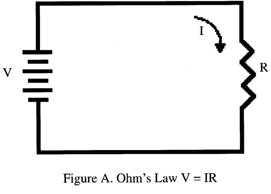
Just about every component designed to operate in an automobile was designed to run on a minimum 12 volts. When this voltage, V, is applied across a resistance, R, a current, I, will flow in the closed circuit. Measuring the voltage across a load really presents no problem for most installers - simply place the probes of a volt meter across the load and read the answer. The current in the loop can also be measured, and since Ohm's law tells us that V = IR, the resistance can be easily calculated. See Figure A.

It has been our experience that determining the current flowing from a supply into a load and back out of that load into the supply is not exactly straightforward for many installers. Whenever a problem occurs in a system, the power source needs to be checked. Overloading a power supply by drawing too much current in a load will surely cause the power supply to fail. I've often heard installers state that their particular load was drawing 10 amps only later to find out that this figure was indicative of the fuse in the circuit and NOT of the current flowing in the loop. (Fuses are usually for short circuit protection and do not necessarily represent the actual current.) How then can current be accurately measured?

And finally, we have the quantity of resistance. For a given voltage, the amount of resistance in a circuit determines exactly how much current will flow through that circuit. But how do we measure resistance? Many installers think that resistance can be measured just like voltage and current. Well, let's begin with voltage and work our way down this list.

Measuring Voltage

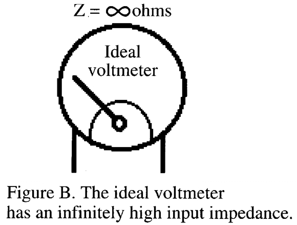
The ideal voltmeter draws no current and has a very high input impedance. In the old days, we were happy if our voltmeters exhibited 10,000 ohms/volt. Modern DVMs (Digital Volt Meters) often have input impedances of over 100 Megohms (100,000,000 ohms). See Figure B.

Voltmeters read across the circuit or load under test. This means that typical readings are taken with the circuit in operation. In fact, it would be meaningless to measure the voltage across a load that was not in operation because the result should be zero volts. Right? There is, however, validity in measuring the open circuit supply voltage as well as the supply potential when under load. This measurement will tell us just how much the load is effecting the supply.

Forty years ago, the mechanical D'Arsonval meter movement was the accepted standard. With this type of meter, higher voltages created greater meter movements. Various voltage scales were simply voltage dividers that permitted the same meter action to be used for many different ranges. When measuring transient waveforms, the D'Arsonval movement tended to average the voltages and provide a good representation of the actual potential. Modern DVMs do not work in this manner and tend to display varying numbers when evaluating complex waveforms as the samples are flashed across the display.

Measuring alternating current (AC) with the D'Arsonval movement required little more than passing the signal through a rectifier and then reading the DC value. However with DVMs the signal is typically fed into integrated circuits (ICs) known as Analog to Digital converters (A-Ds). With AC, many values are commonly calculated, including: peak-to-peak, average and RMS. Remember, when working with AC, it is important to know what value the meter is actually reading.

Measuring Current

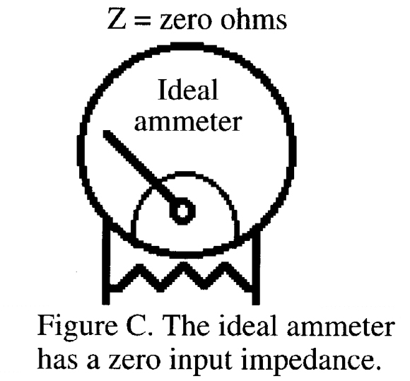
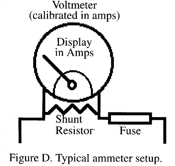
The ideal current meter (ammeter) has zero input impedance. In fact, it should represent a short circuit. An ammeter is always placed in series with the circuit to be measured. This is why an ammeter with a very low input impedance is desirable - so that it will have a minimal effect on the circuit under examination. See Figure C.

Ammeters work by measuring the voltage dropped across what is known as a shunt resistor. Clip on ammeters work on a slightly different principle, but, they can be accurate to within approximately 2% and are easy to use. To measure the current flowing in a particular closed circuit, the circuit must first be broken and the ammeter must be connected in series. When the circuit is reactivated, current will flow through the ammeter's shunt resistor causing a voltage drop across the resistor. This voltage drop is then displayed on a voltmeter that is calibrated in amps. It is important to use a fuse in series with the shunt resistor whenever the amount of current is largely unknown. The fuse will protect the shunt resistor from damage in the event the current range is exceeded. Seasoned installers will always set the ammeter to its highest current range, and then progressively move down the scale until the proper range is found. See Figure D.

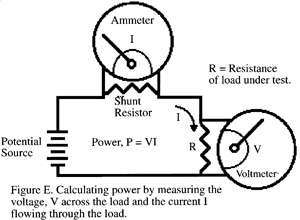
Measuring Power

To measure power, both the voltage across the circuit and the current flowing through the circuit must be known. This does not usually present us with too much of a problem for steady state DC, but with the varying phase relationship between the current and the voltage in AC circuits, accurately measuring the power can be a little tricky. Typically power meters are used with frequencies under 1000 Hz.

With two meters, the measurement of power in DC circuits can be straightforward. See Figure E.

Turn-on triggering circuits have long been a sore subject in a few brands and models of components. For instance, if the input resistance of a turn-on sensing circuit is too high, then just about any stray voltage can activate the circuitry. On the other hand, if the input resistance is too low, excessive current will flow in the circuit and possibly overload the source. Almost always the source of turn-on current is a semiconductor device with limited output capability. In some extreme cases the amount of current available at the "electric antenna turn-on output" was found to be less than 50 mA. Now remember, semi-conductor devices are usually associated with a voltage drop of their own. This means that there will normally be less than the input voltage available at the output of a transistor-switched device. Don't forget that as the voltage goes down, the current must increase to perform a given amount of work.

When installers try to connect loads, such as a typical automotive 12 VDC, 30-Amp rated contact, automotive relay, the current requirement of the relay's coil often exceeds the 50 mA limit. The result can be a burned trace on the deck's PC board, a "blown" resistor, or a damaged semi-conductor device. Measuring the power consumed by the load would have made this problem trivial, but how many installers ever bother? Instead, many decks were returned to the factory for repairs. (In this particular case, most of the decks were retrofitted with high current Darlington switches capable of driving several automotive relays.) See Figure F.

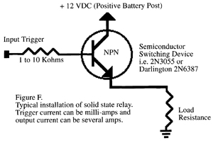
Another problem here is when several components are connected in parallel to a single turn-on lead. Does it make good engineering sense to design several amperes of current to be sourced from a deck? Anyway, the point is to check the load requirements of a circuit before connecting it to what may, or may not, be an unlimited source of power. The obvious solution would be to use a solid state switch or relay as a buffer between the deck's turn-on output and the inputs of the rest of the components.

Measuring Resistance

Resistance measurements are done internally in the meter by using a battery to supply current to the resistance under test. The current flowing through the resistance is then measured by its associated voltage drop and the result is displayed as resistance by the meter. It is very important that the battery supply is the only current flowing through the resistance under test. If outside currents happen to flow though the resistance, then the meter cannot accurately measure the resistance under test.

There have been a few occasions in car audio in which exceedingly low resistance measurements have been published. We're talking on the order of .001 ohms. These measurements were supposedly meant to qualify various ground points on the chassis of a car. But since we usually experience noise only when the engine is running, then shouldn't we be making our measurements at the same time? With ground currents flowing all over the chassis of a car, such readings are totally useless because the circuit under test was active and not totally passive. Resistance must be measured with no current flowing except the current from the VOM (Volt Ohm Meter). This is a fact of life for us car audio installers.

Taking accurate low resistance readings in a car is a difficult task. Although it can be done, the accepted engineering method is to use the resistance between any two points on the car as the shunt resistor and then to measure the voltage drop across the resistance with something like a laboratory-grade amplifier. But who really cares? As soon as the engine is started, ground currents will begin flowing all over the car. These currents often wreak havoc with our car audio components and are the real source of our problems. For instance, taking many low resistance readings (.001 ohms or so) with the engine off is of little help in removing alternator whine from a component with poor power supply isolation. And on the other hand, with the engine running there can be no serious resistance readings taken on the chassis of the car because current will be flowing. Over the last 15 years, many installers have "debugged" their systems by taking resistance readings with the engine running. I can even remember a couple of guys that discovered "negative resistance." It seems that their meters were moving in negative direction because the circuit under test was active rather than passive. Totally meaningless readings.

Another source of aggravation for the novice installer has to be the measurement of a resistor that is soldered into a circuit. Unless one end of the resistor is un-soldered, that resistor just may be connected to other resistors, or capacitors. By the way, charged capacitors in parallel with resistors always make for interesting resistance readings. At A2TB we have had installers call with reports of changing resistance values on the order of factors of 1000. Resistance must be measured with no current flowing - except the current provided by the measuring system itself.

Types of Meters

From a practical standpoint, a couple of good analog meters of the type manufactured by Simpson or Triplett work just fine for most installation applications. We highly recommend picking up a meter like this at a swap meet or garage sale. The shunt fuses are easily accessible and the ranges are clearly defined. I recently visited an alarm shop that had customized their meters by installing circuit breakers on the test leads and then shorted across the shunt fuse receptacles. Replacing a shunt fuse with a circuit breaker is not a good idea because it can severely alter the accuracy of the reading. DVMs have long caused problems for some installers. The problem is that the input impedance of such devices is often so high (so as to not effect the circuit under test), that useless numbers rapidly flash across the display. We have had installers call in with reports of alternator induced voltage spikes on the order of 200 volts. That may be true, but such spikes do not necessarily mean that the alternator has bad diodes or that the alternator is going to explode and ruin the entire electrical system of the car. The response of an analog meter would not let quick spikes register a meter movement. It is important to know the limitations of your test equipment.

One last thought on meters for use in car audio applications would be cost. Over the years, we've lost many meters. It is far better to lose a moderately priced meter than an expensive full featured meter. We'll cover more on this subject in future issues.

---

A2403 - Current and Efficiency

By Richard Clark

It is very common to see installers adding up all the fuse sizes contained in the components of a system to arrive at the total system current draw. Using this technique almost always results in power calculations that are unrealistic. On many occasions the huge number that results is the justification for "an alternator upgrade."

"High Output" Alternators

As anyone that reads our newsletter knows, we are categorically against upgrading alternators. Seldom are they really needed. More often than not, changing alternators causes secondary problems related to the function of the vehicle. As cars become more and more complicated and charging systems become even more integrated into the vehicle, "upgrading" alternators may not even be possible. Only a few short years ago large alternators and multiple batteries were the norm in high-end car audio. These electrical behemoths were usually connected together with another unnecessary product. This device was the diode isolator. From the very first issue of A2TB, we took a hard stand against electrical systems built around so called "high output alternators," second batteries, and diode isolators. Nevertheless, in an industry that is slow to accept change we feel that our influence has been positive. Most large car audio systems of today rarely include larger alternators and more than two batteries. And the device that was designed to work in campers and RVs, the diode isolator, has all but disappeared from car audio. Only the technically unenlightened still adhere to these antiquated techniques.

System Current Requirements

We still get a lot of questions from new subscribers about total system current draw. If the system is anything other than a multi-thousand watt SPL creation, our answer is always the same “Don't worry about your alternator, everything will be just fine, trust us.”

Even so we still get an occasional, "How can this be?"

After all, it only seems natural that totaling the combined fuse sizes would be a good indicator of electrical consumption. This is certainly the way we would do things if we were going to wire a building or determine the requirements for more conventional accessories on our vehicle such as running lights or a winch.

We thought it might be a good time to explain the most underlying reason that a seemingly large system that is sometimes fused in the hundreds of amps can usually be accommodated by most car electrical systems. Let's start by overlooking the most obvious reason. That would have to be that you aren't going to listen to your system at full volume 100% of the time. This simple fact would easily explain why you might not need to have all the calculated power capacity. On the other hand we want to be able to turn things up and not experience problems. After all that is why we chose such a big system in the first place.

Listening to Music

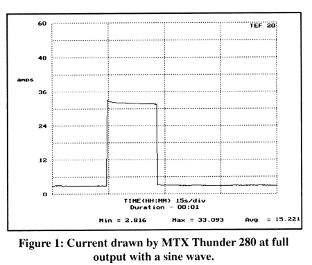
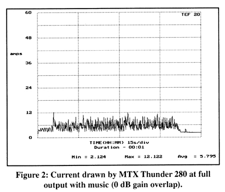
The reason we don't require the reserve capacity that is indicated by the fuses in our amplifiers has to do with the nature of music. Music by its very nature is constantly changing. These changes are both in frequency content as well as amplitude. Let's examine the effect that this can have on an amplifier. Figure 1 shows the current drawn by a MTX 280 amplifier driven to full output into a 4-ohm load. The power output level was about 280 watts. The chart shows current drawn over a one-minute period. The hot idle current was about 2.8 amps, and when the signal was applied for about 15 seconds, the current draw went up to about 33 amps. This amp comes with a 30-amp fuse and if we want to produce nonmusical test tones at full volume, then this fuse would be about right. All fuses can handle more than their face value for a modest time without any problem.

Now if we want to play music, the facts appear totally different. Because nearly all music has a crest factor of more than 10 dB, the average power produced by an amp when playing music is significantly less than it is when playing test tones. To demonstrate this fact we took the same amplifier and fed music into the same 4-ohm load. We raised the level of the music until clipping was just observed on the very highest, but brief, music peaks. This level would be the absolute highest level you could play with minimum distortion. There would be no gain overlap, i.e. the peak input voltage was equal to the amp's input sensitivity - in this case it was 2.4 volts.

Figure 2 shows the actual current drawn by the same MTX 280 amplifier under these conditions. Even though the amplifier had brief musical peaks that reached full output (280 Watts), the peak current drawn by the supply only reached a maximum of about 12 amps. Overall, the average current drawn was only about 6 amps! This amplifier only needs a fuse of about 8 to 10 amps to play continuous music right to the point of peak clipping. What is even more important here is that the load reflected on the car's electrical system is also represented by this current demand. Far short of the 33 amps represented by our sine wave test.

How Can This Be?

Many installers are confused by the fact that we said the amplifier actually delivered full output yet at no time did the peak input current exceed 12 amps. A simple calculation (amps x volts) would show that if this were true, the amplifier would be delivering 280 watts and only consuming 168 watts. Of course the laws governing the conservation of energy would not allow this to happen.

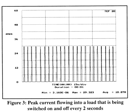
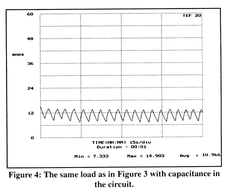
In order to understand this power input/output concept, we need to study the integration of power at the input of a switching supply that contains a large amount of input capacitance. To illustrate what happens when capacitance is involved in a circuit that is switching power compare Figure 3 to Figure 4. Figure 3 shows the peak current flowing into a load that is being switched on an off at a rate of about once every couple of seconds. The transitions are very sharp and go from maximum to minimum very quickly. In Figure 4 we see the same amount of power being switched, but there is a considerable amount of capacitance involved. The charge and discharge associated with the energy storage of the capacitor in the circuit causes the transitions to be more gradual. The peak current demands are averaged over a longer time period and therefore represent the same amount of average energy - even though they don't reach the same absolute values of Figure 3.

Energy Integration Over Time

In the example of Figure 2, the momentary musical peaks where the amplifier outputs 280 watts, a large portion of the energy is sourced from the internal supply capacitance and the energy is quickly replenished between musical peaks. This is what we mean when we speak of the energy integration over time. If we were to calculate the total average energy input versus the total average output, it would be seen that the energy input would greater than the total energy output. The ratio of input power to output power represents the efficiency of the amplifier. Any power that enters the amp and doesn't exit as power to drive the speaker is dissipated as heat inside the amplifier.

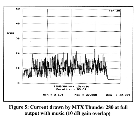
Now let's return to the MTX 280 amplifier. If we increase the drive voltage to the amplifier until the signal peaks provide about 10 dB of gain overlap (signal voltage at three times the maximum unclipped input sensitivity), we will be at the point where distortion will just be noticeable with most program material. As we have recommended in other articles, this is usually the best compromise between distortion and loudness.

The Autosound 2000 Level Setting CD #104 was designed to make this adjustment quick and easy. When the system is adjusted according to these guidelines it will play nearly 10 dB louder. Of course the power requirements of the amp will increase accordingly. Figure 5 shows the increased current demands under these conditions. Even with this increased drive condition, the average current demands of this amplifier are only 13 amps and the highest peak was 27 amps. The duration of this highest peak was so short (fractions of a second), that it would not even blow a 10-amp fuse. Most fuses of the type used in amplifiers don't blow until they are loaded with more than their rating for several seconds.

An Extreme Example

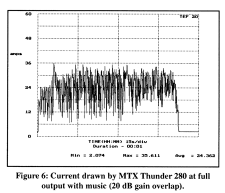
Although our last test represents the maximum anyone concerned with sound quality would ever push their amp, we thought it might be good to show an extreme case. In Figure 6 we show the current drawn by the MTX 280 when it is driven so hard that the signal is totally distorted. The input voltage was over 10 times its rated sensitivity and the music was almost indistinguishable. Not even with these conditions did the amplifier draw continuous current to equal what it did under sine wave conditions. The average current was only about 24 amps. There were momentary peaks that reached 35 amps.

What these simple tests show us is that with music it is not possible to consume current from the car's electrical system in amounts anywhere near the amp's typical fuse size, provided we listen to normal music. Fuses are usually sized to protect the amplifier under extreme fault conditions and rarely are an indication of the current consumed under normal operation. It is for this reason that judging system consumption by adding fuse size is such a misleading approach.

Need assurance? Then try an experiment. Replace the power supply fuses (not speaker fuses) in your amplifiers with a value that is about one third the standard value. Chances are you will not be able to blow those fuses until the system reaches intolerable levels of distortion.

Amplifier Efficiency

While we are covering the subject of power consumption and how it relates to real world operation, it seems appropriate to mention the subject of efficiency as it relates to amplifiers. If amplifiers actually consumed current at the rate implicated by their fuse size, I would be a lot more concerned about efficiency. Because the speakers that are always used with amps are several orders of magnitude less efficient than even the most inefficient amplifiers, I don't normally concern myself with the subject of amplifier efficiency. (Recall that speakers are rarely more than 1 % efficient.)

Still some people really place a great importance on the amp efficiency specification. Unlike a lot of other specifications that are quoted for amplifiers, measuring efficiency doesn't require expensive test equipment. With an inexpensive DVM and a current probe or even a simple current shunt, the efficiency of an amplifier can easily be measured.

By using Ohm's law we can calculate the power going into an amplifier and the power coming out of that same amplifier. The ratio is the efficiency. When measuring the efficiency of an amplifier it is important to realize that the efficiency will vary with the signal level and even the frequencies reproduced. With some amplifiers the efficiency can vary with the voltage of the power supply. As a general rule, the efficiency improves with higher power supply voltages and higher output levels. It turns out that the output level has a very large effect on efficiency. The higher the output levels the more efficient most car audio amplifiers become.

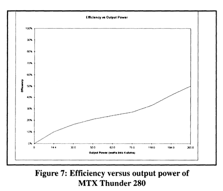
To show the efficiencies achieved with actual amplifiers we have plotted the efficiency versus output level of the MTX 280 that was used in the previous tests. The test frequency was 1 kHz and the amplifier was bridged into a four ohm load. As is typical of all amps, the efficiency at lower levels is very low. Less than 10% is not unusual. Of course, the actual power consumed at low levels is low so this is nothing to worry about.

As the power output increases, the efficiency usually goes up. Amplifiers are most efficient when they are at full power and right at the threshold of clipping. When comparing the efficiency of amplifiers it is very important that the specs are compared on the same part of the power curve. Amplifiers that produce more power than their rated spec will look less efficient than they really are if this factor is not considered. The MTX 280, for example, is rated for 160 watts at 4 ohms. A look at Figure 7 will show that at 160 watts it is about 40% efficient. This amp however actually produces over 260 watts in this mode. If we rate the efficiency at its true output, then we can see that it is really 50% efficient.

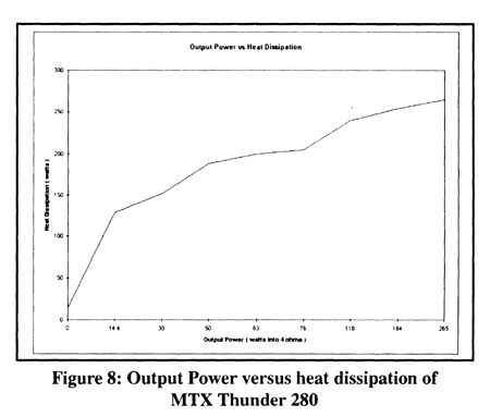
To get a clear picture of what this really means in terms of heat dissipation see Figure 8. In this chart we have plotted actual heat dissipation in the amplifier at different power levels. The heat rises rather quickly until about 1/3 power and then it begins to level off.

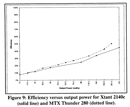
We recently received an amplifier from a subscriber for testing. We were told that the manufacturer claimed that it was about 70% efficient. The amp was an Xtant 2140c. When compared to the MTX 280 it was actually less efficient on a watt per watt basis. See Figure 9. Because of the fact that the output power of the Xtant (320 watts bridged into 4 ohms) was higher than the MTX 280, the power curves do not line up and therefore the efficiency numbers should not be directly compared.

70% efficiency? No Way!

Still the Xtant amplifier looked pretty ordinary for an amp that was claiming to be 70% efficient. Considering that efficiency is such an easy spec to verify, we thought it strange that a reputable manufacturer would make such an overstated claim. The book and literature that came with the amp mentioned that there were some special characteristics of the power supply that made it very efficient so we thought we would check it out a little closer.

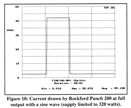
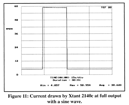
It seemed that a direct comparison with another amp would be in order. We wanted to make the comparison as fair as possible. To do so requires that we compare the Xtant amp to another amp of the same power range. We needed an amp that produced about 320 watts when bridged into 4 ohms. Every amp we had on hand produced either more or less power than this amp. To solve this problem we used a Rockford 200. When powered at 14 volts the Rockford 200 amplifier actually produces over 450 watts when bridged into a 4-ohm load. Because the Rockford supply is unregulated, the power of this amp can be reduced by simply lowering the supply voltage. We found that if the supply was lowered to exactly 11.54 volts, then the Rockford 200 amp produced 320 watts ---- exactly the same as the Xtant 2140c when it was powered with 12.8 volts.

When reproducing a 1 kHz sine wave at 320 watts into 4 ohms, the Rockford 200 amp consumed 50.6 amps of current at 11.54 volts for an efficiency of 58%. The result can be seen in Figure 10. To produce exactly the same amount of power, the Xtant 2140c actually consumed 59 amps of current at 12.8 volts for an efficiency of 45%. So the much-touted efficiency of the Xtant 2140c turned out to be less than the Rockford 200 and considerably less than the advertised claim of 70%.

Some Music, Please

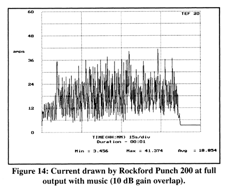
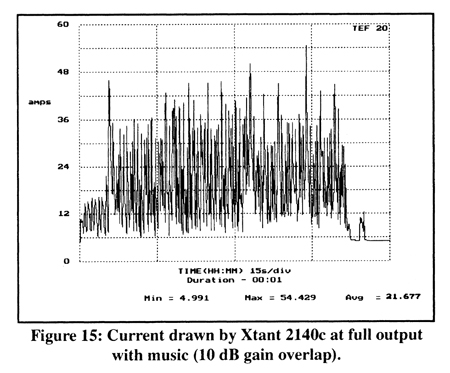
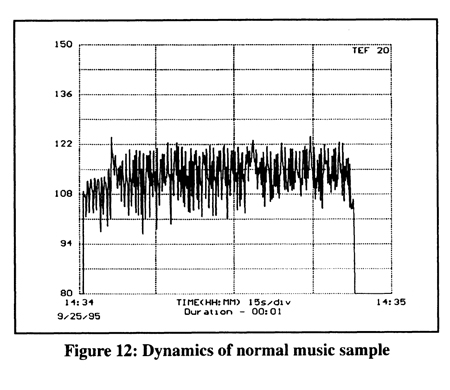
Considering the fact that the Xtant amp fell so short of its efficiency specification, we thought that perhaps we should test it with music instead of test signals. There are some power supply designs that can track music signals and optimize certain parameters for best operation under changing conditions. Both amps were adjusted so they were at exactly the same level and so that the peak music program material just reached clipping. Figures 12 and 13 show the results of this test.

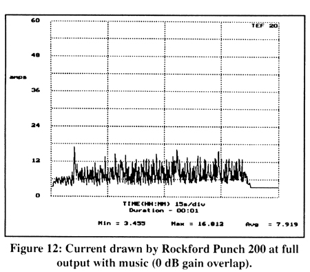
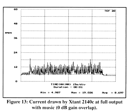
The current drawn by both amplifiers is displayed for a period of about one minute. The average current drawn by the Rockford 200 was 7.9 amps and the Xtant 2140c consumed 8.6 amps. To calculate actual efficiency with such a signal is very difficult and complex because the average power for the same time period has to also be monitored. Even though we don't know the actual efficiency numbers, it is easy to see that whatever they are, the Rockford 200 is more efficient than the Xtant 2140c.

We also did the test at elevated levels. With 10 dB of gain overlap at the input, the current drawn can be seen in Figures 14 and 15. The Rockford drew an average of 19 amps with peaks as high as 41 amps. The Xtant drew an average of 21 amps with a peak of 54 amps.

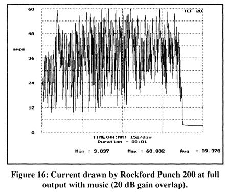
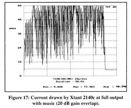
With the amps driven very hard (terrible distortion), the current consumed can be seen in Figures 16 and 17. The Rockford consumed an average of 39 amps with a peak of 60 amps. The Xtant went way off the 60-amp scale for much of the measurement and drew an average of 48 amps with a peak of 74 amps. In each of these last tests, the peak current exceeded the maximum current consumed by the same amps for an undistorted signal because the energy of the clipped waveform was so high. The total peak output of both amplifiers probably exceeded 500 watts, but the signal was too distorted to be usable.

Winding Down

Ok, so amplifier fuses are only for catastrophic protection and should not be viewed as a representation of the actual current consumed by the amplifier. Amplifier efficiency is not a particularly important specification in light of the intended purpose of an amplifier - to drive a terribly inefficient electromechanical speaker. A more useful efficiency specification might to measure the amp-speaker combination. Amplifier efficiency is easy to check and our readers should not be over impressed with advertised claims that are not substantiated. This is one of the reasons for the new A2TB component certification program. To add honesty to component ratings with no partiality to advertisers, marketing departments, friends, etc.

---

A2404 - Dynamic Range and Loudness

By Richard Clark

In order to reproduce music faithfully, it is necessary for a system to reproduce as large a dynamic range as possible. Before the use of electrical recording techniques, the recording needle actually had to move a small diaphragm that was attached to the throat of a tulip shaped horn. The maximum volume was limited by how far the record groove could move the needle. Electrical recording was certainly a giant breakthrough in this respect.

Next, the record pickup produced an electrical signal that could be amplified to any level to produce the desired volume. Tape recorder heads also reproduce small electrical signals that can be amplified as well. However, the extra volume that was achieved with electrical gain was not without its problems. The electrical gain required to make a large volume of sound from the tiny record undulations, or the playback currents of the tape head, also increased the level of noise reproduced by these mediums.

To reproduce good dynamic range requires not only a high volume capability but also a low noise floor. In fact, dynamic range is specified as a ratio in dB from the quietest sound to the loudest sound a system is capable of. When all of the recording mediums were analog the dynamic range of a system could be improved in two ways. The noise floor of the system could be lowered, or the recording level could be increased. Anyone who has ever bought a blank tape remembers that everyone claimed to have "lower noise" and "higher output". The dynamic range of a modern recording system can be very large indeed. Modern digital recording systems are capable of nearly 100 dB of useable range.

Unfortunately, because of the way many modern recordings are made, most of this technical advancement is wasted. Many modern recordings actually exhibit very little dynamic range. The reason for this is that people often confuse loudness for dynamic range. I recently overheard a group of competitors discussing a disc they felt to be really dynamic. They loaned the disc to me to get my opinion and when I told them it wasn't dynamic at all, they were confused. And, when I told them they needed a CD with minimum dynamics to demonstrate how loud their system would play, they were totally confused.

Modulation Envelopes

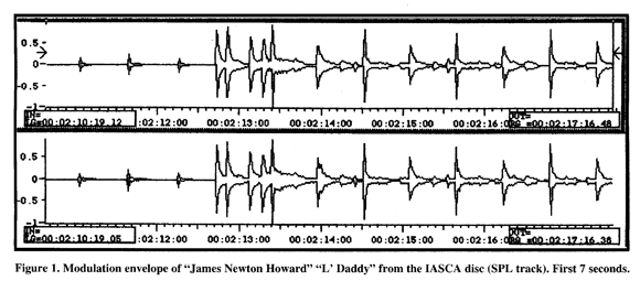
To clarify this issue, let's explore a measurement known as the modulation envelope. In this type of display the vertical axis indicates energy. The horizontal axis is in units of time. A typical display might look something like Figure 1. This display shows the energy content of a song from a CD. The horizontal scale lasts for 7 seconds. The vertical limits are equal to the maximum level that can be recorded on a CD. This is a condition known as "all high bits." This song just happens to be the first seven seconds of L' Daddy, which is track 4 of the Sheffield Lab disc titled James Newton Howard. Most of you will recognize this as the SPL cut from the IASCA CD. Notice the three small blips that are actually the opening three counts of the drum sticks slapped together. Notice that three seconds into the song the recording has already reached 100% modulation or all high bits in both channels (the upper envelope is the left channel and the lower is the right).

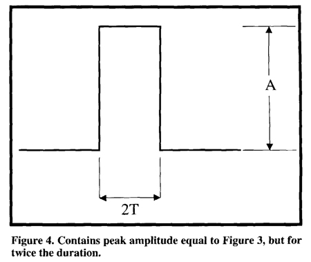
Now let's pretend that we are a recording engineer and we want to make a louder CD. Unlike in the days of analog recording where we could go back to the chemical lab and invent some new kind of ultra high output magnetic particle, the digital system has preset limits that can not be exceeded. With digital recording there is absolutely no way to exceed 100 % modulation. The only choice we have to increase the perceived loudness of the recording is to decrease the dynamic range! This would amount to increasing the quieter parts of the music to increase the overall energy level. The modulation envelope of such a recording will typically look like Figure 2. This display shows the first 15 seconds of Bass Creations Vol 5, track 4 "Funky Low Bass." Notice that the maximum levels are not any higher (they can not be), however, the average energy levels are greatly increased. In engineering terms, we would say that the "area under the curve" has been increased. For example, the following waveform, Figure 3, exhibits an amplitude and duration. Let's say that the amplitude is equal to A and the duration is equal to T.

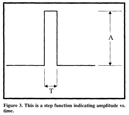
Figure 4 is similar to Figure 3, and has the same amplitude, A, but the duration is equal to T times 2. The total energy represented by Figure 4 is twice that of Figure 3. Interesting enough, it takes just as much amplifier power to reproduce Figure 3 as Figure 4, even though the total energy has a 2:1 ratio. Figure 4 will probably sound louder to our ears even though the maximum SPL is the same! The reason for this is because our ears, like a SPL meter, have a definite response time and the sensitivities are time weighted.

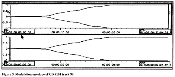
In the future we plan to do a lot of articles related to loudness measurements so that we may understand them better. For now, a basic understanding of the modulation envelope is fundamental. Figure 5 shows the modulation envelope of a track from CD #101. The slowly increasing volume of track 99 is easily seen as is starts at 0% and goes all the way to 100% modulation. Figure 6 shows track 30 of CD #102 for the first 7 seconds. Notice it has less dynamic range than even Bass Creations Disc #5.

It is this reduction in dynamic range that makes something sound loud to the ear and this is exactly why radio stations usually compress their broadcasts. They are willing to suppress the dynamic range in order to make their station sound louder. Many popular recordings are processed the same way. The natural dynamics that are so important to good reproduction are sacrificed to increase the overall perceived loudness. This is the reason higher quality recordings sometimes do not sound as loud when compared to over-processed, overproduced recordings.

The only way to increase dynamics in a digital format is to lower the overall recording level in order to allow more room for peaks to be reproduced faithfully with no level compression or distortion. It is for this reason that so much emphasis is being placed on improved low level resolution in digital formats. Unfortunately, at very low levels, digital systems exhibit their greatest short comings.

Remember two things, 1) it is the changes in music that make it dynamic and exciting, and 2) the loudest possible recording is a square wave at "all high bits." Certainly not very interesting, but very loud and with no dynamics. When it comes to loudness in cars, unfortunately, the cars that are really loud always have exaggerated bass. If the response of the car is uneven and the modulation peak occurs where there is a dip in the response, the overall measured output will be low. Likewise, if the spectral content of the modulation peak occurs where there is a peak in the response, the measured level will be exaggerated. Of course, the duration of the low frequency sounds is usually longer, therefore giving our ears, as well as an SPL meter, a chance to react to the level.

To those of you who are really interested in SPL measurements, stay tuned to our upcoming studies. You will find them interesting and enlightening.

---

A2412 - Damping Factor

By Richard Clark

At a recent AUTOSOUND 2000 manufacturer sponsored seminar, we were asked to comment on the subject of amplifier damping factor. I was extremely surprised to find how much importance was attached to this single specification. Since most folks are a little unclear as to the true meaning of damping factor, we're presenting the following article.

First of all, let's discuss the items that enter into the damping factor calculation. At the heart of this calculation is the output impedance of the amplifier. Most all-modern feedback type amps are of the variety known as constant voltage. This means that they will deliver a constant voltage regardless of their load - at least in theory. Sooner or later the limits of the amplifier's design will prohibit its constant voltage characteristics.

It is this constant voltage output characteristic that permits modern car audio amplifiers to deliver more power into a 2 Ohm load than into a 4 Ohm load. A perfect amplifier should be able to double its power every time its output load is halved. Remember, Power = E x E divided by R. As an example, examine the following chart:

8 Ohms = 25 Watts

4 Ohms = 50 Watts

2 Ohms = 100 Watts

1 Ohm = 200 Watts

.5 Ohm = 400 Watts

.25 Ohm = 800 Watts

.0125 Ohm = 1600 Watts

If an amplifier were theoretically perfect, then it would be capable of the type of performance described in the chart. However, there are many factors that influence this capability. First there is the power supply section of the amplifier. Even if an amplifier had an unlimited power supply with output transistors that could handle the current, the design would still not be able to achieve the theoretically perfect output. The reason being that we do not have access to theoretically perfect components.

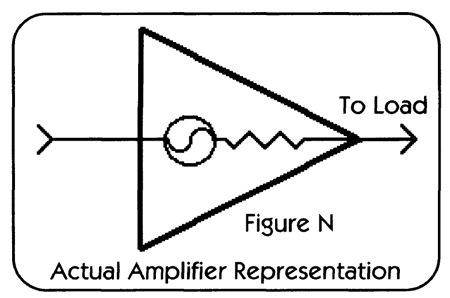
Never lose sight of the fact that real components in real amplifiers are subject to real losses. These losses are a result of junction losses; IR drops in connections and losses in resistances and reactance. Losses in the output stages essentially form a voltage divider on the output of the amplifier. This drop is always in series with the load and can be indicated as in Figure N.

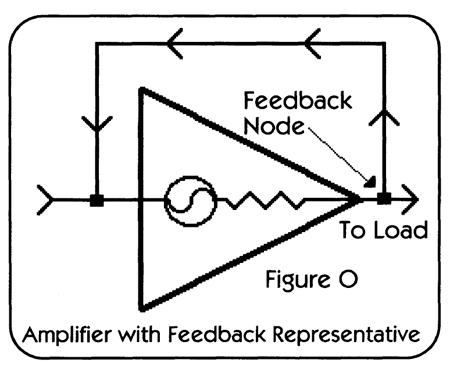
In the design of an amplifier, the feedback network is usually wrapped around the section with the most losses. These losses can be greatly minimized due to the fact that the feedback node is constantly being corrected. This can be depicted as in Figure O.

Output Impedance Determines Damping Factor

If the output impedance of an amplifier is extremely low, the effect of loading on the output of the amplifier will be minimal. This means that it will not experience a voltage loss across its own output impedance. This output impedance does more than determine the effect of loading on the amp. It also determines its damping factor.

Whenever a signal is fed into a loudspeaker the cone of the speaker will move. Since the cone has mass, there will be mass in motion. Mass in motion means momentum. When the signal is removed from the loudspeaker, the momentum of the cone causes the energy stored in the cone to be fed back into the amplifier. If our perfect amplifier were connected to this speaker, the loudspeaker would be trying to produce a voltage into 0 Ohms. Remember, a perfect amplifier has an output impedance of 0 Ohms which is essentially a short circuit.

A voltage cannot be developed across 0 Ohms because it would require an infinite amount of current. It is this same infinite amount of energy that would now be trying to prevent the speaker cone from moving. If such were the case, we would certainly have a "tight" sounding speaker with absolutely no hangover.

The good news is that quality amplifiers have very low output impedances. We are very pleased to report that there are many car audio amplifiers on the market with output impedances on the order of .01 Ohms or less!

Calculating Damping Factor

Let's clarify a few points before starting our calculations. The frequency of the measurement and the impedance of the load need to be specified. For example, the use of a 1 KHz signal and a load impedance of 4 Ohms would be a typical specification.

DEFINITION

A good definition of damping factor would the ratio of the output impedance of the amplifier to the impedance of the load specified at a given frequency.

An amplifier with an output impedance of 0.5 Ohm will have a damping factor of 8 when connected to a theoretically perfect 4 Ohm loudspeaker (i.e. purely inductive voice coil.) since 4/.5 = 8.

The following chart assumes such a 4 Ohm speaker:

Output Impedance 4 Ohms 2 Ohms 1 Ohm .5 Ohm .25 Ohm .125 Ohm .062 Ohm .031 Ohm .0015 Ohm .0007 Ohm .0003 Ohm .00015 Ohm .00007 Ohm .00003 Ohm

Damping Factor 1 2 4 8 16 32 64 128 256 512 1024 2048 4096 8192

Now, for the bad news; it is easy to see how a race to produce such a high damping factor led to a specification so often quoted by salespeople. The numbers on modern amplifiers (with lots of feedback) can get very large and they are easy to compare. Sometimes we can get caught up in these big numbers and we totally miss the point.

Effective Damping Factor (EDF)

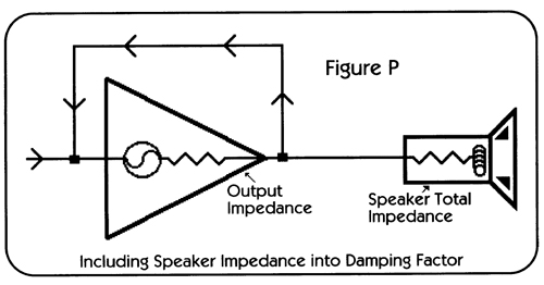
In the case of damping factor, I believe that it could be compared to the old saying of not being able to see the forest because of all the trees. The only thing that really matters is Effective Damping Factor (EDF). Effective Damping Factor more accurately describes the interaction between a real amplifier and a real speaker. Unfortunately real speakers have a real problem with EDF. This is due primarily to the DC resistance of the voice coil. When we calculate the EDF of an amplifier and speaker, it is absolutely necessary that we include this DC resistance into the formula. Figure P illustrates the inclusion of the speaker's impedance into the EDF.

The actual impedance of the speaker may be 4 Ohms. If we measure the voice coil of this speaker, we will probably find that it has a DC resistance of about 3 Ohms. When calculating the EDF effect on this speaker, we must add the 3 Ohms of DC resistance as if it were a resistor between the output of the amp and the voice coil of the speaker. Remember the resistive part of the speaker is the part where the signal is turned into heat. No work is actually done in this resistance.

The inductive element of the voice coil is the only part that does work to create sound. This is one reason speakers are so inefficient. Most of the voice coil is a resistive element that can do no work. Someday if we develop room temperature superconductors and can afford to use them for voice coils, we are going to see some really efficient speakers.

From the damping factor chart it is obvious that the most damping we can expect from our amp/speaker combination is only about two. An amplifier with a damping factor exceeding 10 times this amount is no longer going to play a significant role in this overall calculation. This would yield a practical limit on amplifier damping requirements to about twenty.

There are times when the actual damping factor can exceed this number; one such case would be that of a dynamic loudspeaker in resonance. As we have learned, at resonance a loudspeaker's impedance is at a maximum level. At resonance, the DC element stays the same and only the reactance increases. This means that the ratio gets larger and the DC element becomes a smaller percentage of the total.

For example, if the speaker impedance at resonance increased to 40 Ohms and the DC resistance was still 3 Ohms and the amplifier were .1 Ohms, and then the actual damping could be 40/3.1, or 13. This is certainly much better than 2, but quite a bit short of the 100, 200, or 500 claimed by salesmen who unknowingly think this factor so important. Fortunately for most loudspeakers this extra damping happens where they need it the most. This is because at resonance, speakers typically are very uncontrolled and have the least mechanical damping. It is also this factor that enables us to be able to connect speakers in series and not have to worry about losing damping. The actual impedance of the loudspeakers in series is doubled, but the ratio to the amplifier must also be increased by a factor of 2 to 1. The result is no change in performance.

It is quite possible that this information may be in stark contrast to current marketing trends. However this does not change the fact that this information is accurate. The best way to achieve total control over speaker movement is with a servo system. Only armed with a quality servo system can effective damping characteristics be achieved. A servo essentially puts the loudspeaker in the corrective feedback loop of the amplifier. This topic will be the subject of a future article.

---

A2414 - Peak Performance

By Richard Clark

Are you having trouble finding available space for extra 12-volt batteries for your sound system? Have you considered the extra weight, maintenance, and safety hazards associated with a large multiple battery installation? Well, there may be another solution at hand that can provide the extra energy necessary to win your next contest.

There is another elementary circuit element capable of storing vast quantities of direct current. This circuit element was first called the Leyden jar, then a condenser, and now is known as an electrolytic capacitor. By virtue of its unique design, a capacitor can store lots of energy.

Because a capacitor typically has many times the plate surface area of a battery, its internal impedance is very, very low. A capacitor can deliver extremely large amounts of current in a very small period of time.

Power Supply Requirements

Have you ever noticed your headlights dimming, or your sound system fizzling out when trying to reproduce explosive transients? It is possible that the battery supplying energy to your sound system is suffering from the voltage drop that is inherent to all lead-acid batteries. This voltage drop is due to the internal resistance of the battery. (It is this same internal resistance that dictates a higher than 13-Volt charging system to maintain a battery)

By paralleling more batteries, the overall internal resistance can be lowered, but if you are only interested in improving the performance of your sound system there may be no need to add extra batteries. Adding more batteries can, however, increase the amount of time that you can listen to your sound system with the engine off.

Batteries have very high current ratings, but when required to deliver large amounts of energy, it is not uncommon to find that the instantaneous output will drop several volts. This is easily measured with a storage oscilloscope and cannot normally be seen on a typical digital or analog voltmeter.

Fortunately, car stereo sound systems rarely consume power continuously. High quality car audio amplifiers operate with switching power supplies. This means that your amplifier is not really driven by 12 VDC, but actually pulsed DC. High frequency pulsed DC actually exhibits a lot of the same characteristics of alternating current, such as being limited by the series inductance of the battery and associated power cables. The switching frequencies typically used in high quality power amps are usually in excess of 30,000 Hz. This means that your sound system really needs 30,000 high current pulses per second to power the amplifiers that drive the speakers.

A Water Tank Analogy

Let's compare a storage battery to a 1000-gallon water tank. At the bottom of the tank there is a 2-inch water line (amplifier's power wire) leading to a faucet. Somewhere on this 2-inch water line is a restrictor, which can be thought of as the equivalent of the internal resistance of the storage battery.

Ok, so far? Next, let's install a 10 gallon water can about 15 feet away from the 1000 gallon tank. The 10-gallon can represents a large value electrolytic capacitor. At the bottom of the 10-gallon can let's install a 6-inch pipe and a 6-inch valve. This pipe and valve will permit the 10-gallon can to empty its contents very rapidly.

When the little faucet is opened, water flows from the tank into the amp, which is represented by a tub in the drawing. Also, when the big faucet is opened, lots of water flows into the amp. Now when the amplifier (tub) requires water, the largest amount of water will be supplied by the 10-gallon can - not the 1000-gallon tank. This is because it has less restriction (i.e. impedance) in its path. This quality is inherent in the internal construction of the capacitor.

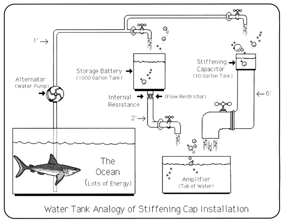
By the way, the alternator is represented in our analogy by the water pump and the ocean would serve as a virtually infinite supply of water.

Stiffening Capacitors

Quality capacitors chosen with low ESL (Equivalent Series Inductance) and ESR (Equivalent Series Resistance) can be paralleled with your existing battery to stiffen its regulation characteristics. When selecting a capacitor for use in a vehicle, it should exhibit a minimum working voltage of 20 Volts (peak 35 Volts) and should have a temperature rating suitable for the installation location. The ideal place to mount your stiffening capacitor is as close to the amplifiers as possible.

The stiffening capacitors must be connected in parallel with the battery supply of the amplifier(s). Also they should be connected to the amplifiers with very large leads. Make sure the polarity is correct because a big capacitor is the equivalent of a hand grenade when connected backwards. Get it right the first time.

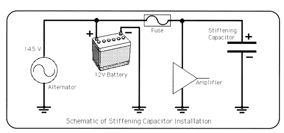
And how big a capacitor is required? Capacitor energy storage is like money in the bank ---- you can't have too much. Here is one of the few places in car audio where more is really better. Values in the one Farad range (that's 1,000,000 mfd) are not uncommon. A good recommendation would be 1 Farad per 1000 Watts of amplification. If you find difficulty in locating the value of capacitor required for your system, remember that capacitors in parallel permit individual capacitor values to be directly added to form one large value.

As far back as 1983, Wayne Harris (of Rockford Fosgate fame) installed a trunk full of parallel capacitors in his first National Crank-It-Up Contest winning entry. Today, large value capacitors are readily available from Monster Performance Car in a size and with added features for any system.

As with any 12- Volt connection in the vehicle, take all precautions to insulate and protect all exposed leads. Also keep the power leads as short as possible. Remember, the whole purpose of doing this is to eliminate the series resistance between the power source and the amplifier.

Testing the System

The music content most to benefit by the installation of the stiffening capacitor is strong transient sounds such as drums or plucked strings. At high levels the transient accuracy and overall definition of the sound system has been demonstrated to be greatly improved.

Our tests have shown that if alI batteries are up front in the engine compartment where they are safe, warm and able to charge under ideal conditions, then a rear installed capacitor, or capacitor bank, will eliminate the negative effects of having the amplifiers mounted a great distance from the energy source.

---

A2420 - Distortion and Speaker Damage

By Richard Clark

The subject of speaker damage is always a high interest topic in car audio circles. Because many of us tend to run our speakers close to the edge, the possibility of damage is greatly increased. A good understanding of why speakers actually fail can be of great benefit to designers, installers and operators of audio systems. It is unfortunate that there is so much misinformation about this subject. Because certain aspects of the subject are very complex, it is no wonder that there are so many explanations floating around.

Some of the aspects of speaker damage are rather easy to understand. Mechanical failure due to certain physical related factors is obvious. For instance, poking a hole through a cone with your foot doesn't take much of a study to evaluate. Wrecking a speaker because it moved so far that it literally ripped its suspension and cone apart is also a common mode of failure. Many woofers that are used in poorly designed boxes have met this fate. Tweeters without adequate crossovers have also seen a lot of failures due to over-excursion.

Thermal Failure

Although for this article we don't intend to cover such obvious modes of failure, there is one that we want to cover. This is known as thermal failure. As the word implies this failure is a result of the temperature of the speaker getting too hot. It would seem that the cause of this should also be obvious, however, after talking to many consumers, subscribers and manufacturers, it seems that this failure is not clearly understood.

After hearing some of the explanations for the actual causes, I am no longer surprised that it is so common. It seems that there are a lot of technically unfounded theories as to the cause. We felt it was time to clear up some of these myths! When we say that a speaker "burned up" we are usually referring to the fact that something in the speaker actually got so hot that it burned up. Just like any other object that burns as a result of getting too hot, certain components in a speaker will actually burn up rendering the speaker useless. These parts are usually the voice coil and the former that it is wound on. Too much electric current flowing through the coil causes the heat. Just as with a hair dryer element or light bulb that glows when current flows through it, the voice coil of a speaker will also get excessively hot if the current exceeds a certain amount. This amount is determined by several factors. The size of the wire can matter. The larger the wire the more current it can handle. The type of insulation on the wire can have a big effect. Some types of insulation are more temperature resistant than others.

Even the shape of the wire can matter. Certain shapes such as flat ribbons can allow more exposure to cooling surfaces. The former that the coil is wound on can be made from anything ranging from paper to metal and can greatly influence thermal limits. The type of glue used to hold the parts together can have different resistance to temperature. Some of the more modern epoxies have the remarkable ability to withstand high temperature.

Regardless of how the speaker is made, there is always a limit to the power it can safely handle without damage. It is usually in defining this power limit that we have a lot of confusion. When we rate an electrical device we use the term watts. Some electrical devices are easy to rate. Take for example a light bulb. When we rate a light bulb at 60 watts, we know that 60 watts of power will flow continuously through that bulb as long as it is turned on. If we increase the power by a significant amount, the bulb will burn up because its filament will get too hot and melt. If, we reduce the voltage to the bulb then the filament will cool off and the light will become dim. As long as the voltage and current remain within the design parameters of the bulb, it will work as intended. With a constant source of power it is easy to rate the power capacity of a component.

Speaker Power Rating

If we were to rate a speaker the way we do a light bulb, it would be easy to arrive at a value but that number would be useless considering the way we use our speakers. Unlike AC line voltage, music signals are constantly changing. If we look at a typical music signal over a short period of time we will see that there are peaks that are several times as large as the average level. When we consider the power of such a complex signal, the actual values of the waveform must be integrated over a given time period. It is the total power under the curve that determines the power, therefore the heating, of the signal.

For an example of this examine the following charts. The measurements were taken from the speaker terminals of a power amplifier. Each chart is a display of power for a period of one minute so each vertical division represents 15 seconds.

Figure 1 shows a constant power level of a 1 kHz sine wave. For the entire one-minute measurement period the level shows no variation. This continuous signal is similar to the 60 Hz that a light bulb would see. Figure 2 shows the levels that are typical of music. The levels can be seen to vary over a range of about 20 dB. The interesting fact about Figures 1 and 2 is that when the music is averaged over the period of one minute, it represents exactly the same power level as the continuous sine wave. The highest power point in the music selection is near the start of the song and is nearly 10 dB louder than the average level. This high point is in contrast to the lowest point that occurs about 20 seconds into the song. The lowest point is about one tenth the average power (about 5 watts).

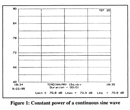
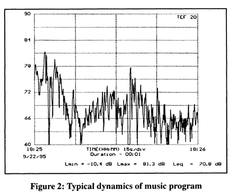
If the continuous sine wave of Figure 1 were used as a reference and played at a power level of 50 watts, it is easy to see the heating effect that would occur in the voice coil of a speaker. What is not always understood is that if the signal of Figure 2 were played into that same speaker, the heating effect would be the same even though there were momentary peaks of 500 watts. If our speaker were rated at a truly honest 50 watts continuous, neither of these signals would cause any thermal damage even though the music had peaks that reached 500 watts. It may cause excursion damage but that is another failure mode.

Thermal Mass

Because the duration of those 500-watt peaks was very short, the voice coil would not have time to actually heat up. To understand why such large power peaks do not damage the coil we have to think of the term thermal mass. Even though the power is high the coil can absorb a certain amount of heat before its temperature starts to rise to unsafe limits. This principal is easily demonstrated with a candle. It is easy and painless to pass a finger through the flame of a candle as long as it is done quickly. This doesn't mean the candle isn't hot. It just shows that the thermal mass of our finger is able to absorb a certain amount of heat before we start to get burned. As long as we give our finger time to cool between passes we can do this repeatedly.

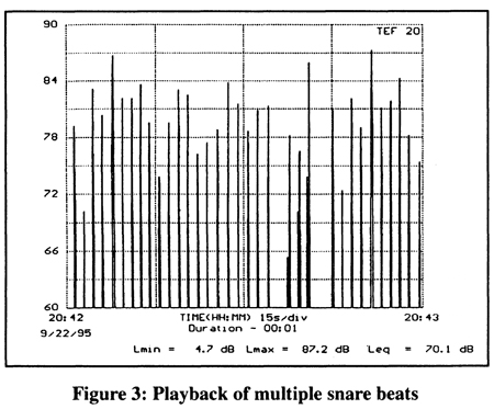
Now for an extreme example of power variation. Figure 3 is a power vs. time plot of a snare drum beat reproduced by a very large amplifier. The average power of this signal was also the same as the signals in Figures 1 and 2. Some of the beats are 17 dB louder than the average level. Seventeen dB above 50 watts is over 2000 watts! If our 50-watt speaker were driven with this signal, it is very likely that it would not be damaged due to the cooling period between the peaks. Even though the momentary peaks are very high, the average power level, and therefore the average heating effect, is only 50 watts.

It is this very nature of music that makes rating the power of speakers so difficult. If our sample speaker could handle 50 continuous watts, we could rate it at that power level. If we were going to play only tones with our system then it would be simple to properly match it to a 50-watt amplifier. If we were going to play music with our system, a quick look at Figure 2 will show us that a 50-watt amplifier would probably not be adequate for our speaker.

The speaker was easily able to handle 500-watt music peaks. If the speaker were matched to a 50-watt amplifier and we tried to play the music of Figure 2 at an average power level of 50 watts, we would find that the amplifier would be greatly undersized for our 50-watt speaker. In such a case we would find that the amplifier would be very distorted during most of the music. Anytime the signals consisted of peaks that exceeded 50 watts, they would be clipped by the amplifier.

Distortion

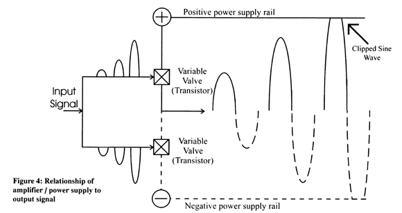
This brings us to an interesting, but often misunderstood, subject: Distortion. Let's consider the fact that all music is composed of sine waves. The combinations of frequencies, amplitudes, and phase relationships are virtually infinite. To keep the explanation simple, let's first consider a single sine wave. Most amplifiers have no trouble passing a sine wave with virtually no distortion. They can do this at all levels up to their maximum rating. The power supply rails usually determine the maximum rating. The rails of an amplifier are the outputs of the power supply of the amplifier and are a DC potential. In modern amplifiers there is usually a positive and negative rail. When the amp is outputting a sine wave, the energy is diverted from these rails by the output transistors that act as variable valves.

As the sine wave swings positive, the energy is diverted from the positive rail and when it goes negative, the energy comes from the negative rail. As long as the voltage required for the sine wave is less than the power supply rail, the amplifier will have no trouble reproducing the signal without distortion. When the signal required is higher than the rail voltage, then the transistor acting as a variable valve is turned on completely and the rail of the amplifier is literally connected to the speaker. This full "on" condition is known as saturation and it occurs for whatever duration of the wave that exceeds the rail of the amp. See Figure 4 for a simplified block diagram of an amplifier and the relative relationship of signals to rail voltages.

Amplifier Clipping

This saturation condition is more commonly referred to by the name that describes what it does to the signal. We call it "clipping." Perhaps no other facet of amplifier behavior is more misunderstood than this condition. Let's cover some of the myths. First it is commonly believed that clipping is bad for an amp. Nothing could be farther from the truth. The transistors in an amplifier operate in a linear mode. This means that for a given current, the power dissipated by the transistor is proportional to the voltage dropped across its junction. When the amp is clipping the transistors are fully saturated and have virtually no excessive drop across their junctions. This places them in their most efficient condition. True digital amplifiers operate in this condition all the time and this is why they are so efficient.

Pure DC?

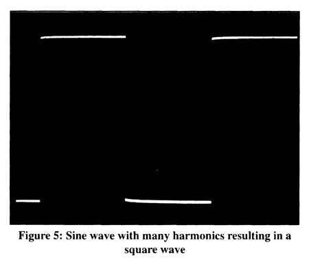
It is also commonly believed that when an amplifier clips that it puts out DC. A quick look may make this appear to be true, but it would have to be a very quick look. Let's take the example of a clipped 100 Hz sine wave. If we examine it for more than 1/200'" of a second, we will see that the signal inverts polarity at the same periodic rate as an unclipped sine wave of the same frequency.

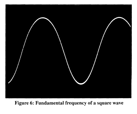
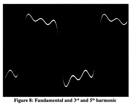
The waveform we are describing is known as a square wave. But wait a minute here; a square wave is not the same as DC. A pure square wave is a complex AC signal that is composed of a fundamental frequency and an infinite number of harmonics. Figure 5 shows an oscilloscope photo of a good square wave. If we examine the makeup of this waveform, we will find that it is composed of many individual sine waves. The first of these is the fundamental. We can observe the fundamental frequency by passing our square wave through a very steep low pass filter. This will remove all of the harmonics and leave only the fundamental. The fundamental is a pure sine wave of the same frequency as that of the square wave and can be seen in Figure 6.

If we move our filter up to three times the fundamental frequency, then we can observe the next harmonic along with the fundamental. This would be known as the third harmonic and can be seen in Figure 7. Moving the filter even higher will reveal more harmonics.

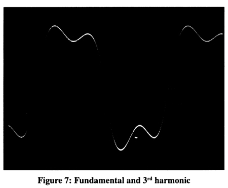
Figure 8 shows the fundamental with the third and fifth harmonics. By the time we add the fifth harmonic the signal starts to resemble the familiar square wave. If we continue to add harmonics, the wave will eventually become more and more filled until it becomes almost square. If you still think clipping is DC and all this seems a little too confusing, we have a little experiment you can try that will convince you that a clipping amplifier doesn't put out DC.

An Experiment into Distortion

All it should take to clear up the DC question is to put a large stiffening cap in series with a speaker. Then hook your speaker to your car battery. No DC will flow because DC doesn't flow through a cap. Now hook the speaker to your amp with the cap in series and turn up your amp until it starts to clip. The clipped signal will go right through the cap. We all know that caps don't pass DC, right? So now that we are on the right track let's get back to the facts. When an amplifier clips a signal, it causes the generation of harmonics. These harmonics are also known by another name. This is what we call distortion. The more an amplifier is over-driven, the more the signal is clipped and the more distortion is generated. No matter how much an amplifier is clipped, it will never produce a perfect square wave because the generation of a pure square wave requires infinite bandwidth. In fact perfect square waves only exist in theory because there is no circuit with the bandwidth necessary to pass one -however, for all practical purposes some of them come pretty close.

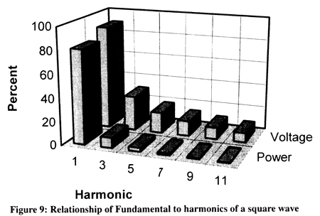
For the interests relating to loudspeaker power capacity, it is only necessary that we concern ourselves with the very basics of square waves. We have already seen the frequency content of a square wave. When a square wave is compared to a sine wave of the same peak amplitude, the square wave will have twice the energy of the sine wave. This is because there is more area under the curve but not all of that extra energy is from the harmonics. If we examine the actual power contained in the individual frequencies that make up the square wave we can see this more clearly.

Figure 9 shows the relative power content of a square wave. The power levels relative to the fundamental decrease with each ascending harmonic. If we add the total energy of the fundamental sine wave with the harmonics we will get a total of 100% of the energy. What is important when we are considering the heating effect on a speaker is that the fundamental frequency of a square wave, which is a sine wave, will contain 2 dB more energy than a sine wave with the same peak voltage as the square wave. Put another way, the fundamental of a square wave has a higher peak (27% more voltage, 62% more power) than the square wave itself.

More Power?

Analysis of this subject can get rather complex but what it really boils down to is that almost any amplifier can produce twice its undistorted output if it is allowed to clip excessively. This extra energy results in about 2 dB more energy at the fundamental and one dB in harmonic content.

It also is commonly believed that there is a difference between square waves that are recorded in program material (such as might be found in heavy metal music) and square waves that occur as a result of amplifier clipping. This is simply not true at all and an understanding of just what makes a square wave should make this clear. By the time we have reached the third overtone (also called the 7" harmonic) the power level is diminished to only a couple of percent of the fundamental. A whopping 8 % of the total power is still contained in the fundamental.

If we are concerned about power dissipation in speakers it is easy to see that we need not concern ourselves with harmonics much beyond this point. How the signal is generated is not important at all. The only thing that matters are how much energy the waveform contains. This is the only factor that determines the heating effect on the voice coil of a speaker. It has been suggested that clipping can destroy tweeters. This is seldom the case. If only 19% of the energy is contained in the upper harmonics, then this doesn't really leave us with much destructive energy.

Take the example of the case of a passive three-way system with crossover points at 100 Hz and 2000 Hz. Suppose we clipped a 50 Hz signal going to the woofer with a 100-watt amp. We know that the amp can produce 200 watts of square wave power. Looking at Figure 9 we can calculate that we would have 162 watts (undistorted) of 50 Hz, 18 watts of 150 Hz, 7 watts of 250 Hz, 3 watts of 350 Hz, and 2 watts of 450 Hz. By the time we reached the frequency range of the tweeter, the power would be fractions of a watt. If our system had a tweeter with a power rating of only 10 watts, it is unlikely that adding another fraction of a watt would make much difference.

These harmonic levels represent the absolute worst-case conditions for a single frequency and do not account for the fact that program material contains complex frequencies, all of which clip simultaneously if the amp is overloaded. But the amount of overdrive needed to clip an amplifier to the level demonstrated is well in excess of 30 dB. For an amplifier with an input sensitivity of 2 volts, this would require an input voltage to the amplifier of over 50 volts! This type of drive voltage is virtually unavailable in car audio products.

Of course the same effect could be achieved by feeding the signal to the amplifier in an already clipped state, something that happens frequently. At any rate these excessive conditions don't really apply here as the dynamic changes in music make it very difficult to continuously clip a signal to such an extreme state. Even when an amplifier is overdriven by as much as 20 dB (10 times the rated input voltage), clipping of the waveform will occur only for about 40% of the total time on music. At this point the music is so distorted that it is virtually unlistenable, at least for most listeners.

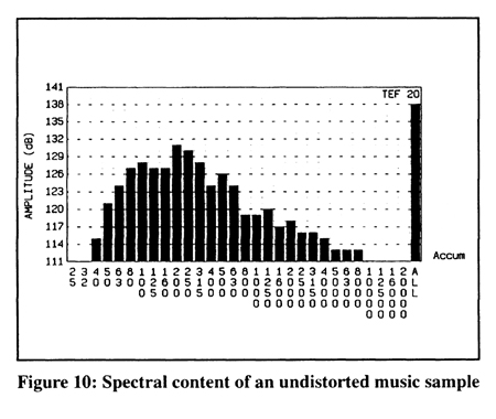
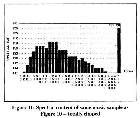
For a demonstration of the actual spectral difference between normal program material and terribly clipped material see Figures 10 and 11. Although the spectrum would be different for different types of music these two curves should be comparable as they were the same piece of music.

Figure 10 is the spectral content of a song averaged over a period of 40 seconds with 243 samples each. Figure 11 is the same song but it is massively clipped. The level was reduced so the curves would represent the same overall level. Notice that the overall spectral content is very similar to the original. These tracks are from our new amplifier level setting CD#104 and are Tracks 31 and 35 respectively. The total energy represented by both tracks is exactly the same and will produce virtually the same heating effect in the voice coil of a speaker. The speaker doesn't care if the music is distorted or not. To a speaker it is all just a combination of sine waves. A speaker cannot tell the difference between noise, distortion, or music. It doesn't care what kind of music it is or any thing else about it except how much energy is contained in the signal.

What Really Matters

The real problem for our speaker is that any amplifier can produce more than its rated power if it is allowed to distort and clipping is a sign that you have probably reached the point where you should turn things down. To get a real picture of what the speaker sees compare Figures 12 and 13.

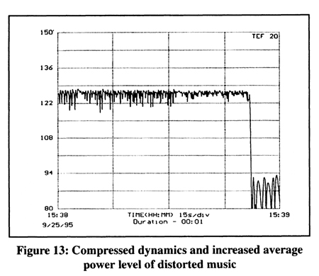
These represent the power vs. time of a song with very steady energy. They are in stark contrast to the song in Figure 2 at the beginning of our article. Figure 12 is the output of an amplifier driven right to the verge of clipping but not quite. The amplifier was a MTX 4160 that is capable of producing about 219 watts (AM certified) per channel into 4 ohms. Even though the peak power to the speaker is over 200 watts the average power is only about 20 watts.

Figure 13 is the same song and the same amplifier, but the gain has been increased until the amp is clipping very severely. Notice that the dynamics (ratio between loud and quiet passages) have been compressed and that the average power level has increased by about 15 dB. Now the average power level is about 100 watts and the peak power is about 400 watts. This means that our speaker is getting five times the heating effect that it was receiving before we started clipping the amp.

Prevention

It is sometimes claimed that a good way to prevent speaker damage is to use a larger amp. This is true only if you don't turn the larger amp up until you exceed the average power to the speaker. A larger amp will allow for the larger transient peaks to be reproduced without damage to the speaker because the total heating of those short peaks is minimal anyway. This will almost always result in a cleaner sounding system. But if you continue to increase the power to the speaker until the average power is excessive, then it doesn't matter if the signal is clean or distorted ---- the speaker will overheat and burn up. Usually when this is done the speaker will begin to distort before the amplifier. If this happens this is a sure sign that you are feeding the speaker too much power.

When considering speaker power ratings and amplifier size it should never be forgotten that although amplifiers are usually rated with continuous sine waves, speakers rarely are. When matching amplifiers and speaker power ratings you are literally comparing apples and oranges. This should not normally be a problem as long as we remember how the ratings differ.

The most efficient woofers rarely exceed even 2%. If we put 100 watts of power into a speaker, this means less than 2% of the power is turned into sound and over 98% of the power is turned into heat. The next time you need to be reminded of how much heat 100 watts is just grab a glowing 100-watt light bulb. And just think, not all of the energy if alight bulb is turned into heat, in fact they are more efficient than most speakers!

If your speaker were fed 100 watts continuously it would have to dissipate this much heat from its coil. Not many speakers are really designed to handle 100-watt continuous sine waves, but when rated for dynamic music that is constantly changing (providing cooling periods), a speaker that can only handle perhaps 50 watts continuous sine waves can easily deal with the undistorted output of a 400-watt amp. That's because the average output of that 400-watt amp reproducing undistorted music is probably not over 50 watts.

If you can keep things under control you will be safe with the 400-watt amp. The same speaker that can handle 50 watts of continuous sine waves can probably deal with 100 watts of a totally distorted amp.

In nearly all cases when we see power ratings on a speaker, the manufacturer has taken into account that you are going to be playing music on that speaker. That is why we see ratings on some small tweeters as high as 100 or even 200 watts. This usually means that if the amp is about the same size and not allowed to distort, then the average power will be about right.

It is not that distortion hurts speakers; it is just that distortion is usually a sign that something is too loud. This is also why we can find examples of 300, 500, and even 1000-watt woofers. You can be sure these are not ratings for continuous sine waves, continuous music maybe, but not sine waves. Next time you think you have a 1000-watt woofer, think about the heat produced by your hair dryer and imagine that much heat building up in a small box in the back of your car! Better get a fire extinguisher!

---

A2491 - Oscilloscope Waveforms

By David Navone and Carl Miller

The advantage of using an oscilloscope is, of course, that one can see and measure exactly what is occurring electrically in a circuit in real time. (Digital storage scopes permit us to dissect the past, but we will save that topic for a future article.) Crunching numbers taken from assorted meter measurements cannot compare to a visual graphic display. From a car audio perspective, a view of an oscilloscope waveform quickly demonstrates the quality and integrity of a "linear" amplifier or any other audio component.

Let's begin our exploration into waveforms, and along the way we will learn how to correlate the display on the oscilloscope with the physical properties of the circuitry under test.

Sinewaves

Examining a sinewave yields excellent results when checking amplitude and phase distortion. One of the first waveforms to be studied with a scope is usually the sinewave and one of the easiest measurements that can be taken of a sinewave would be the frequency. In the past, I have discussed the repetitiveness of motion and how that single quality defined a wave. The time for a sinewave to complete one full cycle is known as the period and it is measured in seconds. The frequency of the sinewave is known as the reciprocal of the period. (This means that f = 1/P, where f = frequency and P = period (in seconds).

By inputting a known sinewave frequency into the scope's horizontal input and then feeding an unknown sinewave into the vertical input we can visualize the relationship between the two: i.e. (2 to 1, 3 to 1, etc.). This can be accomplished by counting the number of peaks in the display. Even before we had oscilloscopes, such measurements were taken with mechanical instruments and smoked plates. Such methods were fine for our grandparents, but today the abundance of inexpensive frequency counters has outmoded this tedious method of measuring the frequency of a particular signal. For illustrative purposes, we included a visual example of this older method in Figure 1. These waveforms are named after the man who developed them. They are called Lissajous waveforms or Lissajous figures.

Dual Channel Scopes

Nearly all of the later model oscilloscopes have two inputs, or channels, for taking measurements. Such scopes are often called "dual probe" devices. Using two probes makes it quite easy to make many comparative measurements ---- particularity phase shift or the delay between two waveforms. See Figure 2 and Figure 3. When we apply a pure audio sine wave to the input of an amplifier (or any other component under test) we usually set the sine wave amplitude for the normal level of the input of the device under test.

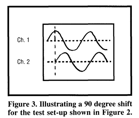
Connect the probe from the scope's Channel 1 to the input of the unit under test and then connect the probe from the scope's Channel 2 to the output of the unit as shown in Figure 2. Using the vertical positioning features for both Channel 1 and Channel 2, position the two sinewaves so that they can be visually compared for a shift in phase as illustrated in Figure 3. One word of caution here is to make sure that the output of the unit under test has the proper load. Without a load the characteristics of the circuit under test may change.

The amount of delay between the input and the output of the component under test can be read on the horizontal axis of the scope. Check the time base settings and make the measurement. Since the time base of most oscilloscopes is calibrated in seconds, milliseconds, and microseconds, some very basic math may be required. To convert the seconds into degrees of shift, recall that one complete waveform represents 360 degrees. A half wave represents 180 degrees, and a quarter wave represents 90 degrees. If a particular output waveform is delayed one quarter of a waveform with respect to the input waveform, then the circuit under test is said to have a 90-degree lagging phase shift.

Change the frequency of the audio signal generator and again make the measurement. Notice how some audio components have a continuously variable phase shift with respect to changes in frequency. For crossovers and equalizers, this is a fact of life.

Single Channel Scopes

If your oscilloscope is not dual channel device, you may test for phase shift by referring to the diagram in Figure 4 and the display illustrated in Figure 5.

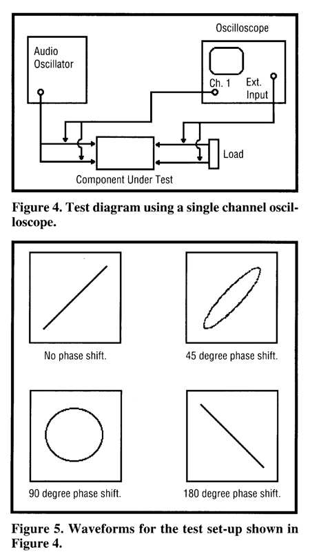
Connect a pure audio sine wave from an audio signal generator to the input of the component to be tested. Adjust the amplitude of the test signal for the proper level at the input and the output of the component under test. The single probe of the oscilloscope should be connected to the input of the unit under test. The output of the component under test should then be connected to the external horizontal input of the oscilloscope.

The vertical dimension of the scope's display can be adjusted by moving the volts/division knob and the horizontal dimension can be adjusted by moving the seconds (or milliseconds) per division knob. The amount of phase shift between the two signals (input and output) can be measured by viewing the resulting waveform. See Figure 5. For our mathematically inclined readers, the formula for calculating the phase angle is shown in Figure 6.

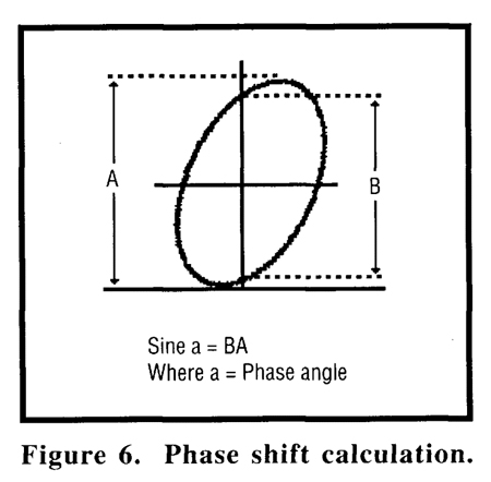
Although this method of determining the phase shift between the input and the output of a device may be somewhat more complicated, it can be just as accurate and revealing.

Square Waves

While a sinewave may be useful in testing something such as an amplifier's performance, it only tells us what is happening at a particular frequency. We usually want to know about all the frequencies within the audio bandwidth ---- and sometimes both above and below the audio bandwidth.

A square wave signal can provide a quick check of an amplifier, or other component, at many frequencies simultaneously. A square wave of a given frequency contains a large number of odd harmonics (the fundamental frequency multiplied by 3,5,7,9, etc.) of that frequency. If a 500 Hz square wave is applied to the input of a circuit, there will also be applied many odd harmonics of the fundamental 500 Hz: i.e. 1500 Hz, 2500 Hz, 3500 Hz, and so on.

Most solid-state amplifying devices are inherently non-linear. Many other audio components are also non-linear because their response to electrical signals is, well, non-linear. To design a perfect component that can provide all frequencies with equal amplification and can faithfully reproduce even the most complex waveform with no distortion and no phase shift is yet to be achieved.

Because a single square wave contains so many frequencies it can quickly reveal even the slightest of problems. Harmonic frequencies as high as the 21st harmonic (21 times the fundamental square wave frequency) must pass through the amplifier in order for the square wave to remain undistorted. Failure of an amplifier, or any other device, to perform in this manner is easily visible with an oscilloscope. Please refer to Figure 2 for the wiring diagram used when performing a square wave test on a component.

Testing With Square Waves

Refer to Figure 7 to view the diagram for square wave testing. The short rise time, which occurs at the beginning of the first half cycle of a square wave, is created by the in-phase sum of all the medium and high frequency sine wave components. Please refer to the waveform illustration in Figure 8. The same holds true for the rapid drop at the end of the first half cycle from the maximum amplitude to the minimum amplitude at the 180-degree or half cycle point.

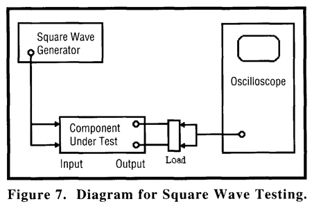
Therefore, a theoretical reduction in amplitude of the high frequency components should produce a rounding of the square corners of the waveform at all four points of one square wave cycle. Figure 8 represents the response of a component with reduced high frequency amplitude and no phase shift. When there is a high frequency loss plus a phase shift, the square wave looks like the drawing in Figure 9A. In the waveform at Figure 9B, we see an overshoot each time the wave changes direction (vertical amplitude). This indicates a high frequency boost in amplitude.

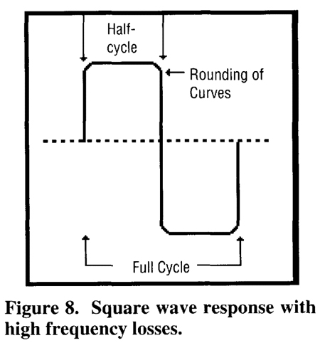
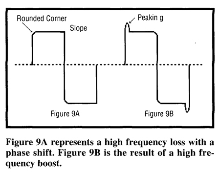
Shown in Figure 10A is the result of a low frequency loss with no phase shift. The waveforms shown in Figure 10B and 10C demonstrate tilts in the square wave. These tilts or slopes are due to phase distortion. The influence of the square wave's third harmonic, either leading or lagging, the fundamental (10B leads, 10C lags) shows up as tilt. Very slight shifts in phase are easily detected by viewing a tilt in the square wave.

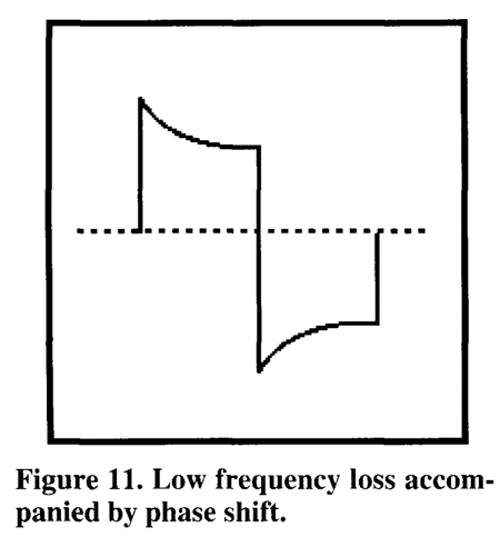
When both a low frequency loss in amplitude and a phase shift occur, the resultant waveform is shown in Figure 11. Low frequency loss is often accompanied by a reactive component (transformer inductance, crossover network, etc.) causing a resultant phase shift. Figure 11 illustrates such a strong tilt.

Figure 11 is a combination of Figure 10A and Figure 10B. It is also true that a combining of Figure 10A and 10C and would appear as the waveform in Figure 11; however, the display would be angled in the opposite direction.

It is a fact of car audio life that various amplifiers, pre-amplifiers, crossovers, and cabling can cause the output of a square wave to differ from the original signal. The important waveforms previously discussed are summarized in Figure 12. Our readers may want to copy and retain this drawing for future oscilloscope reference.

---

A2493 - Polarity and Phase

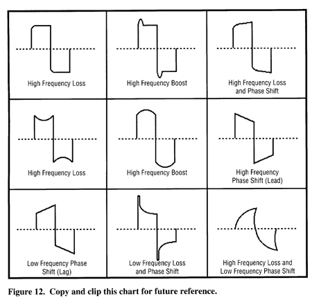
By David Navone

A couple of years ago the owner of a car audio shop called and asked about purchasing a "speaker phase checker." Well, after searching around for a couple of days, it became clear that there weren't exactly hundreds of choices. In fact, we could only find a couple of large pro-audio distribution companies that even knew what we were talking about. Both of these companies were marketing foreign manufactured two-part devices that sold for around $750.00 each.

For car audio that amount seemed expensive in light of the most common method of determining the polarity of a speaker -- the old nine volt battery trick. Did car audio really need a $750.00 tool just to see if a particular speaker's voice coil terminals were correctly labeled? What is so important about the polarity of a speaker? If you're a seasoned installer, just skip down to the section on Crossovers and Phase Relationships. Otherwise, stay tuned for the whole story.

Polarity Defined

We all know that our Earth has a north pole and a south pole. All good boy scouts are aware that the needle labeled "N" on a magnetic compass will always point in the direction of the North Pole. This is because the compass needle has been magnetically "polarized" opposite to that of our Earth's north pole. In reality, it is the south pole of the compass needle that points to the North Pole because: "opposites attract".

Dynamic loudspeakers must obey the same magnetic laws of physics as the compass. Let's explore the principles of operation by first stating a couple of more laws of physics. These laws have been known for over 150 years and ALWAYS apply.

Whenever a current is passed through a conductor, a magnetic field will form around that conductor. If the conductor is wound in a coil, the resulting magnetic field will become focused or concentrated. Such a current carrying coil is known as an electromagnet because its magnetic properties are a direct result of the electrical current flowing in the conductor.

From our Earth studies, we know that magnetic fields have two poles; commonly labeled north and south. Recalling that "opposites attract," the converse, "likes repel," would indicate that the north poles of two different magnets would tend to repel each other. These rules apply to all magnetic fields, whether electrical or natural in origin. This means that the north pole of the magnetic field of an electro-magnet will be attracted to the south pole of a permanent magnet.

It is interesting to note that in applied physics, it is very difficult to discuss electricity without discussing magnetism. The two topics are hopelessly linked in both their mathematics as well as their physical properties.

The driving force behind a dynamic loudspeaker is really nothing more than the interaction between an electro-magnet and a permanent magnet. Early loudspeakers utilized two electromagnets because of difficulties with existing permanent magnet structures. When current flows in one direction through the windings of the voice coil, the magnetic poles will attract. When the direction of current flow is reversed, the magnetic poles will repel.

Typically the electro-magnetic coil is loosely suspended near the permanent magnet. If an object denser than air is attached to this movable electro-magnet, then that object will be forced to move along with the magnet, thereby disturbing the air molecules in the near vicinity. This is exactly how a speaker functions.

The polarity of a speaker is simply determined by the labeling of its voice coil terminals. It could also be said that a speaker's polarity is determined by the direction of current flow through the voice coil, or by the direction of the windings relative to the fixed magnetic field, or by the polarization of the permanent magnet. The majority consensus of car audio manufacturers have determined that when the electromagnetic voice coil and its movable cone is repelled away from the permanent magnet and the basket of the speaker, the terminals of that speaker should be labeled as follows: Mark a + or a RED dot on the voice coil terminal that is connected to the source of positive potential that is causing the coil to repel away from the permanent magnet.

By convention, the other terminal is usually not marked.

The Nine-Volt Battery Test

Let's check it out. Obtain a nine volt battery and any old speaker. Notice that the terminals on the battery are usually spaced about the same distance as terminals on the speaker's basket. Convenient isn't it? Connect the positive (+) electrode of the nine volt battery to the voice coil terminal marked with a + or a RED dot. Very quickly connect the negative (-) electrode of the battery to the unmarked speaker terminal. Did the voice coil jump out away from the basket? If so, then your test speaker followed the most common labeling convention.

Now, reverse the battery's electrodes and re-test your speaker. The speaker's cone should now retract in towards the basket. It would be nice to try this experiment on many different speakers to see if they are labeled the same, however we do not recommend such tests. Even a little nine volt battery is usually too hefty a current source to be directed into a small length of #40 AWG copper wire. The results of such tests can often permanently damage the fragile coil of low powered speakers.

Do not even consider using a battery on a tweeter. Even if you could see the cone move, the end result may be ruinous for the tweeter. Richard mentioned that sometime in his past, he remembers using a 1.5 volt AA battery to quickly move a tweeter. However, he certainly wouldn't think of using a battery on an expensive tweeter. Using batteries are NOT suggested for testing the polarity of expensive speakers.

Enough said about the batteries, the point here is that car audio speaker manufacturers usually abide by the same convention. The problem with relying on speaker terminal markings is that there are some home and pro audio manufacturers who sometimes label by the opposite convention. There are quite a few pro audio speakers being installed in vehicles today. A conscientious installer working on a serious system should not necessarily trust the markings on the speaker's terminals. But there is much more to this topic so let's begin to explore the subject in greater detail.

Polarity Problems

There was recently an article published in Popular Science describing how an obnoxious low frequency fan rumble from a neighborhood processing plant was quieted by the installation of speakers in the smokestack. The fan noise was sampled in real time with a microphone that simply inverted the noise and fed it into an audio amplifier connected to loudspeakers. The amplified inverted noise effectively cancelled the original noise by the principle of superposition. (Don't try this at home. The DSP that made this method work probably cost several hundred thousand dollars.)

The two noise signals are said to be out of phase, or opposite to each other, by 180 degrees. Recall that 180 degrees depicts exactly one-half of a circle. Traveling 180 degrees from any point on the circumference of a circle will yield a point directly opposite. Traveling another 180 degrees, in either direction, will always yield the starting point.

In a car audio system, if one woofer is connected 180 degrees out of phase with another woofer, the net effect on the system is exactly like in the noisy processing plant. The operation of one woofer acts to cancel the operation of the other woofer. Another way to think about this concept is consider the fact that one woofer is pushing the air while the other woofer is pulling that same air. If the speakers are alike and driven with exactly the same signal level, then theoretically the net result is no movement of air.

Practically though, since both speakers cannot be installed in exactly the same place, the sound produced by the vibrating air molecules around the speakers can be less than desirable.

Connecting a single woofer, or any driver for that matter, with a polarity opposed to that of the rest of the system, can cause severe problems in the small listening confines of the interior of a car. Correct polarity must be maintained.

Crossover and Phase Relationships

Crossovers are a necessary evil. An ideal speaker system would not require the use of crossovers. Since the program material captured during a live recording session didn't require a crossover network from Mother Nature, it is unfortunate that our present methods of reproducing that material usually require some type of crossover. Let's take a look at the function of a crossover and then touch on why crossovers can cause us problems.

Due to physical constraints, it is not practical for the serious car audiophile to consider a truly "full range" speaker. Back in the days of AM radio, a full range speaker only had to reproduce the bandwidth of the audio output. It didn't exactly take much of a speaker to handle this requirement.

The motion picture industry was the first to discover that crossovers were necessary when trying to reproduce wide bandwidth audio.

When HiFi became popular, it became evident that the increased bandwidth also could not be reproduced with the available technology without dividing the audio output into at least two groups: low frequencies and high frequencies. The low frequencies were applied to slow moving; large cone area woofers and the high frequencies were applied to fast moving, smaller tweeters. The device responsible for dividing the full range output of the HiFi system was called the crossover.

A crossover is basically an electrical filter network composed of a capacitor, and an inductor. (Sometimes resistors can be used in filters, but for the sake of this article we'll forgo this circuit element.) Filters work by manipulating the alternating current timing relationships between the voltage and current of a particular input. In an AC signal the peak voltage and peak current may be "out-of phase" with one another. This means that one may lead or lag the other. When considering an alternating current flowing through a coil, the current lags the voltage. With a capacitor under the same circumstances, the current leads the voltage. The instantaneous power of our filter network becomes the rate of doing work on the charges within that circuit element. This quantity will always depend on the phase relationship between the voltage and the current. (If our readers can follow this logic, we can eliminate a few dozen complex calculus equations.)

Capacitors store energy in the electric field of their plates and inductors store energy in the magnetic field of their windings. Reactance is the opposition of a circuit element to the flow of AC. This amount is not dependent on the resistance of that element. A reactance will work to change the phase relationship between the current and the voltage flowing into the network. The reactance associated with a capacitor decreases as the frequency increases. This means that capacitors tend to pass higher frequencies easier than lower frequencies. On the other hand, the reactance of an inductor is directly proportional to the frequency. This means that inductors tend to attenuate higher frequencies while passing lower frequencies with ease.

By carefully combining various capacitances and inductances in a filter network, the phase relationship of an AC signal can be accurately manipulated. The desired end product is frequency attenuation. The undesired byproduct is an alteration of the voltage/current phase relationship of the signal.

We define the cutoff frequency of a particular filter as the point where the signal's output power is one-half its input power. This number could also be calculated using the current or voltage, but by convention we measure the power.

Multiple crossover filter elements can be cascaded to essentially filter the filter. The result is even greater filtering. Higher rates of frequency attenuation and greater voltage/current phase manipulation are possible with the addition of more circuit elements.

The Ordering of Networks

Audio engineers commonly refer to the degree of a particular crossover filter as its order. The simplest crossover is called a First Order filter and is characterized by a roll off of 6 dB/octave. An octave is a doubling or halving of frequency. For instance a 440 Hz (middle A on the piano) tone is exactly one octave lower than an 880 Hz (higher A on the piano) tone. Also that same 440 Hz is exactly one octave higher than 220 Hz (lower A on the piano).

A First Order filter has a very low rate of attenuation and requires speakers capable of reproducing a broad spectrum. When high and low frequency speakers are connected to the two outputs of a First Order crossover network, more low frequencies will be directed towards the tweeter than with higher ordered networks. This low rate of attenuation places extra demands on the loudspeakers because the speakers receive more energy outside their normal operating bands. This can be especially troublesome to delicate high frequency speakers.

Now for the tricky part. The outputs of First Order networks happen to be 90 degrees out of phase with one another at the crossover point. The phase of the high pass leg will be +45 degrees with respect to the input signal and the phase of the low pass leg will be -45 degrees with respect to the input signal at the crossover frequency. If the high and low outputs of a First Order network are combined, the result is a signal exactly like the input (perhaps a little lower in level). Some good news is that a 90-degree phase difference will produce constant voltage and constant power at the crossover point. Even though the outputs are shifted by a total of 90 degrees the acoustic sum of the two signals can also result in a combined signal that exhibits little difference. This is particularly true when the drivers are physically aligned and close together.

From the standpoint of phase integrity, a First Order network exhibits the best ability to reconstruct a coherent signal. This is simply because the smoother slopes have less overall effect on the signal. However, this doesn't necessarily mean that a First Order network is the best type of crossover because there are many other factors to consider.

Second Order Filters

A Second Order filter requires twice as many components as a First Order filter. Twice as many components cause a further 90-degree phase shift, which causes a sharper rate of attenuation. This means that at the crossover point, a Second Order network exhibits a 180-degree delay between its outputs and that the frequency roll off is now at 12 dB/octave.

What does this 180-degree shift mean for car audio installers? Well, let's take the example of a tweeter and a mid-range driver installed in a door panel. Let's say that the speakers are mounted as close as possible to each other and that they are each driven by their respective outputs from a Second Order crossover. At the crossover point, and in the crossover region, it's a fact of life that the network outputs will be "out-of-phase" with each other. Within this area, their outputs will cancel resulting in a less than desirable situation.

But what if the tweeter's speaker leads were reversed? Its polarity will now be correct with respect to the mid-range driver at the crossover frequency. Conversely, this means that its output will have to be out of polarity the rest of the time.

Because both speakers must cover the same frequency region, some designers choose to reverse the polarity of the higher frequency driver to help compensate for the phase shift caused by the crossover. Conversely, this means that high frequency speaker will be out of polarity throughout its normal operating band. Its phase relationship with respect to the low frequency driver will be shifted 180 degrees.

Other design engineers do not consider this out-of-phase condition to be a problem. This is because the reversed polarity high frequency driver is hopefully the only speaker propagating these frequencies. Still other engineers feel that if the harmonics of a complex waveform are out-of-phase relative to the fundamental, accurate reproduction cannot be achieved.

Second Order networks are very common in car audio because the 12-dB/octave rates can be successfully used with contemporary drivers. Some manufacturers of Second Order networks commonly reverse the leads of the high frequency output to achieve "in-phase" operation near the crossover point.

Some manufacturers do not subscribe to such practices. Many car audio buffs make their own crossovers from raw components. Does your crossover manufacturer address this matter? Do you invert the high output on your own Second Order crossovers?

Third and Higher Order Filters

Third Order filters contain even more circuit elements than Second and First Ordered networks. This, of course, means even greater roll off and even greater phase shifts. The rate for a Third Order network becomes 18 dB/octave and the phase shift between the high and low outputs will be 270 degrees. As in the previous example, if we were to reverse the leads to the tweeter, we can manage to get the phase shift down to 90 degrees. The result is satisfactory filter performance, as far as car audio is concerned.

Higher Ordered networks continue with this pattern. For instance a Fourth Ordered network exhibits a 24-dB/octave roll off and a 360-degree phase shift in the vicinity of the crossover point. Such a rate of attenuation is considered high and can be used to really keep low frequencies away from sensitive tweeters or to achieve deep, deep bass in a sub-woofer system. The 360-degree phase shift between the outputs brings us back to where we started, albeit a delay. Let's delay this topic for another time.

Back to Polarity

So far we've learned that due to the limitations of our current technology, crossover networks, which are really nothing more than electronic filters, must be used to custom tailor specific frequency regions for specific speakers. The filters do a great job dividing the bandwidth between the outputs, but the laws of physics dictate that the process also alters the phase relationships between the outputs. To minimize these adverse effects, the output of the high frequency section of some filters is often reversed. This is analogous to reversing the polarity of the speaker.

Therefore, any time a crossover network is used in a car audio system, a phase shift will occur. Compensation for this shift may, or may not, be selected in the network itself or in the connections from the network to the speakers. The relative polarity of the speakers in a sound system is not exactly trivial when utilizing crossovers.

Determining Relative Polarity

Achieving relative polarity would mean that all the speakers in a system are working together in the most advantageous manner. Achieving absolute polarity would mean that the sound system was reproducing the software exactly like the original recording; the final result is not inverted. The most important aspect of determining the relative polarity of all the speakers in a system is to thoroughly diagram the entire sound system. It is a car audio fact of life that many manufacturers are not at all concerned if their component happens to invert its output(s). Also, many manufacturers are not even able to supply an answer as to their input/output polarity relationship.

That leaves the serious installer in a rather interesting situation. A good bench tech can be a great help in gathering data for the diagram. It is a simple matter to input a signal, such as sine or square wave, into a component and then look at the output on an oscilloscope to determine if the component is inverting or non-inverting.

Pre-amp level signal cables are usually constructed in a non-inverting manner, but again, the serious installer is advised to make sure. The oscilloscope can also be used to check the validity of the RCA cables in exactly the same manner as previously described. Speaker wires should be color-coded for polarity assurance, but we recommend checking all hidden or bundled leads.

The polarity of large speakers can be checked with the nine-volt battery trick, but what about sensitive speakers and tweeters? How about speakers that are already installed behind grills? The answer to these questions lies in the "speaker phase checker" that was mentioned at the beginning of our article. When first presented with either a pressurized or rarefied wave front, such a device is capable of determining the direction of speaker cone excursion.

Speaker Phase Checkers

With a "speaker phase checker" positioned directly in front of a woofer and with a nine volt battery were connected + to + with the terminals of that woofer, the speaker cone should move outward toward the microphone of the "speaker phase checker." This movement typically corresponds to a GREEN light on the indicator. When the battery electrodes are reversed, the speaker cone should retract back into the basket and illuminate a RED light on the indicator of the "speaker phase checker".

A couple of years ago, I designed a polarity-determining device that became known as the Phase Detector. It is currently being marketed by the Rockford Corporation as the PD-1 and sells for around $200.00. To avoid using nine volt batteries, a companion product, the PD-2 was built to produce positive pulses more suitable for both tweeters and preamp level inputs. We also made a pre-recorded cassette tape, PD-TAPE, that supplied many positive pulses for use in systems with cassette decks.

There is an interesting side note on the PD-TAPE aspect of this project. The auto-reverse decks that were common to car audio during the initial tests of the PD-1, did not always account for the reversal of the direction of tape travel. Consequently, many decks inverted the audio when the tape changed directions. Since the PD-TAPES were only 3 minutes in duration, every 3 minutes the positive pulses on the tape became negative pulses on the output of the deck. This presented quite a problem at both ends of the tape.

The Best Way to Insure Correct Polarity

After many attempts to get a few seconds of pulses placed on future test CDs of other manufacturers, a little over a year ago, AUTOSOUND 2000 decided to go ahead and make our own test software. The result is Track 3 of Test CD #101 which is available for $ 25.00 plus $ 2.50 S/H. This track contains many sequences of three positive pulses followed by a single negative pulse. When Track 3 is played on a CD player the output of the player should be three positive pulses followed by a single negative pulse. With Track 3 and Rockford's PD-1, the absolute polarity of a sound system can be checked in minutes.

To determine absolute polarity, all that is required is to connect the speaker level output of the deck to a test speaker in the manner prescribed in the CD player's instructions. Slowly increase the volume on the deck until one of the lights on the PD-1 begins blinking with the gentle speaker pops. With the Phase Detector in position directly in front of the business end of the test speaker and as on-axis as possible, the indicator on the PD1 should blink three GREENS followed by a single RED. This would indicate that the speaker's cone is moving forward towards the microphone of the PD-1 three times before it moves back only once.

If your CD player does not happen to have a speaker level output, then you can skip the previous step and simply check the output of the amplifier at the end of the system. This is really the only valid system test since we are primarily concerned with the polarity of the speakers when they are driven by the amplified, and sometimes processed, pulses on Track 3. Remember, no matter how much amplification and signal processing a system may possess, if a positive pulse is correctly recorded on the software, then the system should exhibit that same positive pulse when reproduced through its speakers.

Problems with Polarity Testing

Working in a laboratory and working in the real world can yield very different results. The hostile reflective environment of the interior of a car can cause erroneous readings unless the technician is fully appraised of all the pertinent facts. First of all, the pulses on Track 3 are spaced far enough apart so that the reflection of any particular pulse has adequate time to decay before the next pulse comes along. That's good.

Problems occur when multiple drivers are checked with more than one driver pulsing. We highly recommend using the balance and fader controls as well as using only one amplifier at a time when seriously checking a system for polarity. In this manner the speakers can be checked one at a time.

Speakers in the dash are sometimes reflected so severely that the initial wave front is at least partially cancelled by its reflection. The solution here is to decrease the volume of the deck and move the microphone of the PD-1 as close to the speaker's grill as possible. In this way the accuracy of the measurement is assured.

There is no harm in performing many tests on the same speaker. If you are not 100% convinced by your results, try doing the tests again. Remember, it is not unusual to discover that your high frequency drivers are connected "out-of-phase" with the rest of the system.

Absolute Polarity

Before the debut of Test CD #101, the best that could be achieved for most of us in car audio was relative polarity throughout the system. This simply means that all the speakers are working together. Although some engineers may believe the subject of absolute polarity to be controversial, if accurate reproduction is to be achieved, absolute polarity is mandatory.

---

A2495 - Power Wiring

By David Navone

At A2000 we get asked to check out quite a few competition, demo, and regular customer vehicles. Sometimes clients drive their cars to our California office and other times they take their cars to North Carolina. No matter what the problem, we usually require at least a schematic or pictorial drawing of the sound system before we start evaluating the situation. Even though the power-wiring scheme is not usually depicted, the installer will sometimes go to great lengths discussing the subject of power wiring car audio systems. Let's discuss the considerations for successful power wiring.

Contesting or Real Life?

At the beginning of every installation there must be a decision made as to how the vehicle will be used. Will the client ever enter a sanctioned contest? If so, then what are the considerations as far as power wiring is concerned? First of all, the rulebooks state that the power wires leading to the positive battery post must be fused within a relatively short distance from that post. We have absolutely no problem with that rule. Eliminating the catastrophic short circuit protection would be foolish.

Next the rulebooks usually list various gauges of wire along with their maximum current carrying capacity. Basically, our amps consume their energy in short intervals rather than continuously. Therefore the wire charts in the rulebooks usually require oversized wire gauges. This is not really a problem. If you're going to a contest, go ahead and use the big stuff.

Our recommendation is that the wire size recommendations of the amplifier manufacturer be followed, unless you're contesting, in which case you'll end up with garden hose sized power cables.

Type of Power Wire

All power wire is not alike. Solid wire, such as that used in house wiring, is definitely NOT advised for car audio installations. Fine stranded copper wire is the item of choice. Usually, more strands in the wire result in a better (more flexible) cable.

The insulation should be approved for automotive applications. This means that the wire is relatively immune to the adverse effects of petroleum products. Remember, the power leads usually get routed to the inside of the engine compartment and can therefore be subjected to gas, diesel, oil, brake fluid, radiator coolant, etc.

We have seen the recent emergence of shielded power wire. What do they think they're shielding against, quark rays from Mars? In car audio, we're mostly concerned with low frequency electromagnetic interference. When someone comes up with an effective shield for that, give the Electric Boat Company a call and have him or her shield his or her next sub. The amount of low frequency attenuation achieved by shielding would be difficult to measure -- even with laboratory equipment.

The Positive Wiring Scheme

Ok, here it is - the A2000 preferred power-wiring scheme. Let's start with the main +12 volt DC power lead. Let's assume that we have a modern, four-door vehicle with the engine and starting battery up front and the amplifiers installed in the trunk. (Since we aren't interested in listening to the sound system for extended periods of time with the engine off, we won't be installing a second battery.)

When the engine is not running, the car’s battery supplies all the energy for the car audio system. This is why we connect our main power lead to the positive battery post. When the engine is started, the alternator supplies virtually all of the electrical energy for the accessories. But rather than connect our main power cable to the output of the alternator, we usually stick with the positive battery post. This is because most factory wiring schemes insure a great connection between the output of the alternator and the positive battery post.

Let's say that we're using around 500 watts of amplification divided between four amplifiers. If we're going to contest, we'll have to use, say #4 AWG (American Wire Gauge) wire. This size is basically jumper cable stuff, but let's do it anyway.

We recommend temporarily removing the ground cable from the car's battery before commencing your power wiring.

1) Begin by using a suitable terminal and connecting one end of the #4 gauge cable to the positive battery post. Take care not to diminish the factory connections.

2) Within 18" of the positive battery post, install a 100-amp circuit breaker or a 100-amp fuse. The circuit breaker is much easier to use and can really help out later when you're making changes to your system. Remember, the exact fuse value is not important here because it is only for short circuit protection of the vehicle in the event of something like a major wreck.

Continuing out of the circuit breaker, route the #4 gauge +12 volt DC power cable inside or under the vehicle and up into the trunk. If the cable is routed under the car, make sure that it is well protected. It is a good idea to use a strong metal conduit if the cable is exposed. The conduit is for protection -- not for shielding low frequency noise!

4) At the trunk, connect the business end of the #4 gauge +12 volt power cable to the common positive terminal of a Stiffening Capacitor. Install as many big caps as is practical because it is the capacitors that will supply the peak energy to your amplifiers by load leveling the demands on the alternator. For this system, we would recommend a minimum of one farad. (You don't need to fuse the Stiffening Capacitor because you already have a fuse at the battery, remember?)

5) Using the shortest possible wires, connect the +12 volt power wires of all the amplifiers to the Stiffening Capacitor. Long, thin wires will increase the inductance and diminish the ability of the Stiffening Capacitor to deliver its energy in quick, powerful, bursts. If you have to externally fuse each amplifier, then go ahead. Many amps are internally or externally fused in the event of meltdown. Leave these fuses in place.

That's it for the main +12 volt DC power wiring. Let's take a look at the negative return.

The Negative (Ground) Wiring Scheme

There are very few engineers who would route long ground leads to anywhere. An electrical ground can be defined as a point of equipotent with all other grounding points. On a car, the conductive metal chassis is the electrical ground for virtually every electrical accessory. Since our power amplifiers feature isolated switching power supplies, we are usually not concerned with sharing ground returns with other vehicle accessories. (Unfortunately, the same cannot be said for poorly isolated pre-amp level components.)

1) Connect one end of a #4 gauge power ground cable to the negative battery post connector. Take care not to diminish the factory connections. (For safety, the negative battery post itself is still disconnected.)

2) Connect the other end of this #4 gauge cable to the frame of the vehicle and as close to the negative battery post as possible. We recommend using star washers, fine threaded nuts and bolts, and a clean metal to clean metal bond. This connection will insure the return to the negative supply.

>3) On some older vehicles, it is a good idea to connect the case of the alternator directly to the negative battery post. Recall GM full sized pickups from 1974 up to around 1990 or so. The alternator bracket was connected with large gauge cable directly to the negative battery post. We particularly recommend this connection if the engine has been replaced. Very few mechanics manage to get all the grounding straps back. Although it may seem like a good idea to connect your main power grounding cable directly to the case of the alternator, for many practical reasons we are reluctant to recommend such a practice.

4) Back at the trunk, connect one end of a #4 gauge power ground cable to the negative terminal of the Stiffening Capacitor. Make sure to use a properly sized ring terminal and a star-type washer to insure a good connection.

5) Using as short a piece as possible, connect the other end of this #4 gauge ground lead to the frame of the car. It is a good idea to locate a trunk grounding point that can be shared with both the car's chassis and frame. Again, use non-corrosive, properly sized and terminated connectors, fine threaded bolts and nuts, and star washers for this procedure. A good length of cable here would be less than two feet. It is a good idea to seal the connection with something like paint or grease.

6) Connect the power ground leads from the amplifiers to the negative terminal on the Stiffening Capacitor. Again, the ground leads must be short as possible and definitely NOT fused.

You can now re-connect the negative battery post back into the system and activate the main power circuit breaker when you're ready.

Notice that we used the chassis and frame of the car as a ground lead. That's because there is usually more conductive metal in the car's chassis/frame than in a long piece of cable, even 0000 gauge cable. The Stiffening Capacitor really supplies the switching power supplies with their energy. Our main purpose is to replenish the cap in between the musical transients.

That's it for power wiring. As always, if your alternator can't keep up with the demands, you'll have to check out a larger model. And if your battery seems to be draining way too quickly when the engine is off, you'll have to add more batteries. However, if you correctly wire your system and plan on listening to musical program material, you may be able to keep your factory alternator and get by with a single battery.

---

A2500 - Speaker Phase

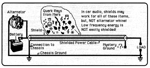
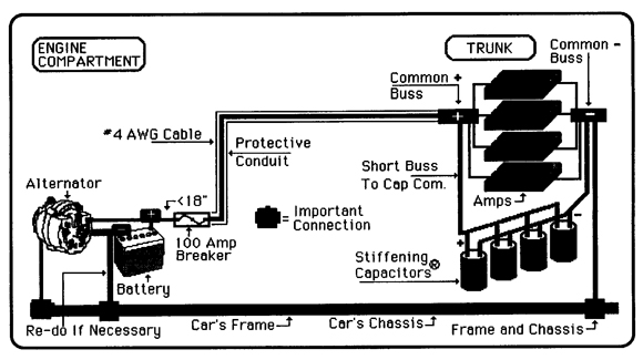
By Richard Clark

Ask most installers if the speakers in his or her car are properly phased and you will probably hear, "Of, course, why would it be any other way?"

Since the plus wire from the amp was connected to the red speaker terminal, the phasing must be correct. Right? Unfortunately, this installer may be living in a dream world where everything is absolutely perfect, however, he or she is installing in a world of imperfect components where Murphy's Law of compounding problems rules supreme. The installer's creed, "If anything can go wrong, it will go wrong," is certainly applicable. Just what can go wrong? Read on.

Amplifier Phase

Some amplifiers are described as being inverting amps while other amplifiers are described as noninverting. A non-inverting amplifier will output a positive signal if a positive signal is fed into its input. On the other hand, an inverting amplifier will output a negative signal if a positive signal is fed into its input.

When all the amplifiers in a sound system are identical, this fact of life usually doesn't matter. However, if there are two amp models or two different brands of amps within the same system, the inverting question takes on monumental proportions. This specification is rarely addressed in amplifier specification sheets. However, it can be easily checked with an oscilloscope.

Speaker Polarity

Most of the time the term phase is mistakenly applied to the direction a speaker moves when driven by an input signal. This is really a description of polarity. The polarity of a speaker may vary from one brand of speaker to another. Some cones move forward and away from the magnet when a positive voltage is applied to their coil terminals. Other speaker cones move backwards and into the magnet when a positive voltage is applied to their terminals. There are even some manufacturers that label tweeters differently than woofers.

While this may be an article on phase, it is impossible to have a system correctly phased until the polarity is absolutely correct.

With large speakers such as midbass drivers and woofers, the polarity can be easily checked with a small flashlight battery. Just apply the battery to the speaker's terminals and observe the direction of motion of the speaker's cone. The speaker will move forward and away from the magnet when the positive battery pole is connected to the + terminal of the speaker. Do not connect a strong battery to a tweeter or expensive mid-range speaker. It may permanently damage the speaker. Use an aftermarket phase checker.

Let's move on to a more challenging subject - speaker phase.

Speaker Phase Characteristics

The actual phase characteristics of a speaker are very complex and somewhat expensive to measure. It may be easy to connect several speakers together and insure that the polarity is correct, however it is very difficult to insure that the speakers are operating truly in phase with each other.

As the radiated frequency increases, phase measurements become more difficult. For example, if we found a perfect loudspeaker, it would project all frequencies with the same propagation delay. This is never the case in the real world. Speakers always tend to radiate some frequencies ahead of or behind other frequencies. This tendency is an indication of the phase response of the speaker.

A typical phase chart would look like the following for a simple single cone dynamic loudspeaker.

See Chart of Speaker Phase Response

The chart should be interpreted as follows. The horizontal scale is measured in frequency (Hz) just like a spectrum analyzer. The vertical scale is calibrated in degrees of phase shift. If the speaker were perfect, then the line would be perfectly straight through zero degrees. If the line ventures above zero, the phase shift is positive and the signals will arrive early with respect to the signals on the zero phase line. If the line dips below zero, the phase shift is negative and the signals will arrive late with respect to the signals on the zero phase line.

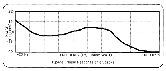
Remember, 360 degrees is equal to one wavelength and phase accuracy gets harder to achieve at higher frequencies. This is because the wavelengths get shorter, and a given amount of offset will equal an increased phase shift.

If absolute accuracy in a speaker system is important, then it is necessary to know the actual phase response of a speaker at a given frequency. If you were going to cross a speaker over at 2 KHz, it is important to know the phase response of the speaker at 2 KHz - not the polarity!

The goal of achieving a smooth phase response determines not only how the speakers should be wired to the network, but also how they should be physically placed within the confines of the vehicle. As one becomes aware of this measurement, you quickly become aware of how difficult it is to achieve good phase response when multiple drivers are used in a system. In this case, less may definitely be better.

Driver placement creates a compound problem. If two identical speakers are mounted side by side and the listener is equidistant between them, their combined direct radiation will be in phase. If the listener moves slightly off center, then he or she will experience a phase shift due to the different path lengths between the speakers and his or her ears.

The shift starts in the high frequencies (shorter wavelengths), and moves down into the lower frequencies as the path length is increased. Remember, this is just the direct sound. What about all the sound that has been reflected from the doors, seats, and windows? The reflections are certainly going to create different path lengths to the listener.

Different path lengths will create multiple destructive cancellations that are directly responsible for so much of the response related problems commonly associated with the interior of a car.

Crossover Problems

It is due to the design of the crossovers themselves that a phase shift is commonly exhibited at the crossover frequency. This fact does not mean that the crossovers are bad; it just means that the installer/technician must allow for this shift. Also, the phase response of the speakers must be factored into the system at the crossover frequency.

It is the sum total phase response that is important and must be compensated for if the system is to have smooth phase response.

This article was intended as an introduction into the very critical subject of speaker phase. In the future, we will address this subject in much greater detail. Stay tuned.

---

A2507 - The Energy Time Curve, or...

(Why 76 Speakers in a Car is Probably Too Many)

By Richard Clark

These days it's unusual to enter into a serious car audio discussion without mentioning the word acoustics. Normally the term acoustics is very loosely applied to the subject of sound quality; i.e. the flavor of a particular dessert is similar to the acoustics of a particular listening environment. We know when the acoustics sound good, but answers as to exactly why and how they sound good can often be elusive.

Acoustics is a term used to describe the behavior of sound waves. Good acoustics would depict the favorable behavior of the sound waves in a particular listening environment. Favorable behavior would be behavior conducive to the enhancement of our enjoyment of the music reproduced within the listening environment.

A thorough understanding of acoustics requires that we study not only how sound behaves within the listening environment (concert hall, home, car), but that we also comprehend the human perception of sound. Unfortunately there is still a lot that is not known about the way we hear and perceive sound. We do, however, know a lot about the way sound behaves in an enclosed space. It is sad that for car audio enthusiasts most of the research dealing with very small rooms, such as cars, has been extremely limited. It is the intention of this article to shed some light on what we know about sound in large rooms (relative) and how that knowledge can be incorporated into the design of a good sounding car audio system.

Direct and Reflected Sound

Let's begin by examining the difference between direct and reflected sound because it is this interaction that forms the basis of what we categorize as the study of acoustics. Whenever a sound is generated in a space, the waves spread out in all directions away from the source. For example, when we are listening to a musical instrument, the first sound we hear is known as the direct sound. Moments later the sound that started out traveling in other directions reflects off the nearby walls and begins to arrive at our ears.

The reflected energy is usually changed as it rebounds from the various surfaces. These changes can be very subtle or very dramatic. The shape, size and surface texture of the reflective surfaces each play a role in the nature of the change. The changes imparted by contact with other surfaces impart an identity signature to the sound wave. Unlike the direct sound that arrived essentially intact and unaltered, the reflected waves may not necessarily resemble their original form.

Our brains are able to process the characteristics of these reflections and yield exceedingly accurate clues as to the nature of the listening environment. For example, if a blindfolded listener were led on a tour of his/her own house, his/her brain would be very capable of accurately determining exactly which room they were visiting. The acoustic clues yielded by a large room are immediately recognizable as very different from those of a small closet.

Our perception of music is likewise affected by the nature of the listening environment. But how does our brain evaluate the data and make such determinations? One common method of studying this subject is to attempt to develop tests capable of measuring data in a like manner. One such test evaluates the energy vs. time relationship.

An energy time curve demonstrates how energy is distributed over a given period of time. A typical ETC (Energy Time-Curve) looks like the following:

The vertical coordinate describes the energy (volume) while the horizontal scale represents the period or time (increases to the right). To read this chart, start at the left and move towards the right. The first major peak will be the arrival of the initial or direct sound. Remember, because the direct path is shortest it must arrive first. After the arrival of the direct sound there is usually a small delay period (well usually) before the arrival of the reflections from around the room.

The reflected energy (remember it is bouncing around the room) will then begin to show a gradual level decay until it eventually disappears. This fade out of energy is known as the reverb time of the room. It is usually labeled as a unit of RT60. This corresponds to the amount of time required for the level of the decay to drop 60 dB.

Many years of experimentation have taught studio designers what works and what doesn't work in a good sounding room. It is universally agreed that after the arrival of the direct sound there should be a time period of at least 10 mS (milliseconds) before the arrival of the reflected energy. It is also agreed that for a good sounding listening room, the reverb time should be on the order of a minimum of .2 to .5 seconds. Uniformity in this reverb range should be throughout the entire audio frequency spectrum. In order for the sound of the room to be considered as good and for the imaging qualities to be stable, a very dense uniform decay becomes extremely important. The good news is that for listeners who are seriously involved in acoustics, the equipment to make these types of measurements has become very reasonably priced in recent years. The bad news is that for car audio listeners the constraints that are considered to be important also happen to be extremely difficult to meet.

It is a fact of life for those of us involved in car audio that the initial time delay, after the arrival of the direct sound, is virtually impossible to achieve. There are, however, many things that can be done to improve the situation. For instance, if the loudspeakers are chosen with respect to a good controlled dispersion pattern and if they’re mounting locations are chosen so as to minimize the reflected energy, it is very possible to achieve a strong initial arrival with a significant reduction of energy immediately following. This absolutely requires that the speakers are not aimed at large objects and that they have an unobstructed acoustic path to the listener.

Another important factor in overcoming the pitfalls of the autosound listening environment is that of the arrival times of the various drivers. It is of paramount importance that all the arrival times be the same. To achieve success under this constraint will require a minimum number of drivers and either physical and/or electronic time alignment.

The next element of concern is that of the reverb time. Until we are able to create the decay characteristics of an ideal listening room, we will never be able to achieve "studio quality" reproduction in a car. Because of the small volume of air contained in a car and the high absorption of the car's interior, the reverb time is extremely short. A typical car audio reverb time will range from a low of about 5 mS to around 60 mS.

Rear Fill

Even if we were able to achieve 50 mS of reverb time in a car, that amount would only be about one fourth of the minimum required of a good sounding room. This lack of reverb time is the reason why some car audio enthusiasts install extra speakers in the rear of the car. When such speakers are properly mounted and driven by signals low enough in level (preferably on a digital delay), they can enhance the effect of ambience that is usually lacking in cars. Ideally, the implementation of such speakers contributes to the often-misunderstood IASCA term "rear fill."

In a good sounding rear filled system, the speakers mounted in the rear of the car should be acoustically transparent. In other words, they should not be noticeable. A good sounding rear filled system should cause the front-seated listeners to sense that there is a large open space to their rear. The word "fill" is used here to refer to addition of reverberant energy to the listening environment. It is this decaying energy that imparts ambience and the feeling of spaciousness into a sound system. If too many rear speakers are used or if they are too loud, the result will be to create more early sound. But this extra early sound will only conflict with the direct sound from the front speakers resulting in wandering and unfocused imaging.

Whenever a sound system contains multiple drivers located throughout the car, the image will suffer. In the next few years, very sophisticated DSP units will be programmed to help in this respect. It is unfortunate that all of the car audio DSP devices that are presently on the market seem to be designed for some, shall we say, completely off-the-path reasons.

Current DSP devices are not capable of fixing poor speaker placement; and may never be. It is also our opinion that crudely attempting to recreate a sound field listening environment such as a stadium or a church is absurd. Maybe someday one of the manufacturers of these devices will finally determine that the ideal environment to recreate would be that of a neutral recording studio at which time the natural ambience in the recording could be reproduced with all of its natural quality. This should be our goal.

---

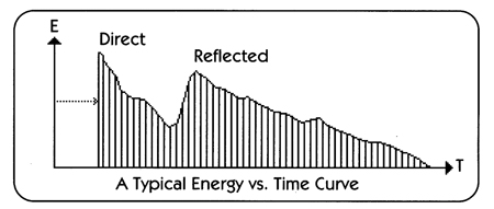
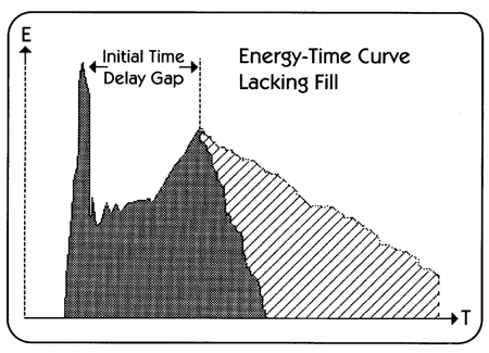
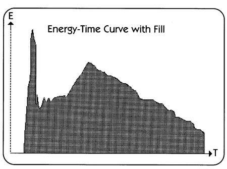
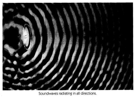
A2511 - The Principle of Superposition

By David Navone

In between sessions at our Seminar/ Workshop in Long Beach, California, some interesting questions came up regarding the propagation of a sine wave from a studio monitor. We had just performed an experiment designed to visualize the wave nature of sound in a rather large listening environment. In one demonstration, a 500 Hz sine wave was produced from a large full range speaker; a hand-held apparatus was used to accurately detect the nodes and crests of the waveform as it "traveled" throughout the auditorium. In this case, the distance between the nodes was measured at around 2 feet and the distance between crests was around 2 feet. When the frequency was lowered even further, the resulting wavelength increased just as predicted.

All went well with the demo, and during a break a couple of interesting questions were asked. First, "How can that hand held apparatus be so accurate when the room is full of reflections and standing waves?" Second, "How can the very same air molecules in the room be used to conduct the incident wave, its first reflections, subsequent reflections, and our public address system as well?"

The answer to the first part of the question is that our demonstration apparatus was carefully designed to compensate for the room acoustics in real time. In essence, the experiment simplified the situation specifically so as to demonstrate the length of a particular sound wave. We eliminated the reflections and concentrated on the initial waveform.

To arrive at an answer to the second part of the question we must look back to the time of Newton. We must look into the work of a Dutch Physicist named Christian Huygens (1629 to 1695). Huygens believed in the wave nature of both sound and light. He was the first audio engineer to conduct studies into how it was possible for the same air molecules to conduct voice, musical instruments, bells, etc., at the same time. Why didn't the various sound waves collide and mutate or destroy each other? The answer is known as Huygens' Principle of Superposition.

The Principle of Superposition

Consider a golf ball dropping into a large pond. The concentric rings formed around the point of impact or the all too familiar crests and troughs characterize origin, P. The crests can also be thought of as the high points of the wave and the troughs would then be the low points. As the wave moves out from P, the leading edge is known as the wave front, W, and it is defined as: The locus of points having the same phase of vibration. Refer to Figure One.

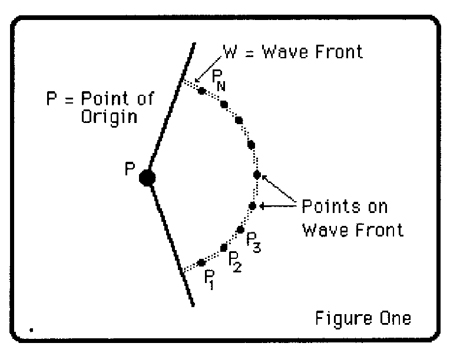
As the wave front spreads out from P, the circumference is always increasing. Huygens proved that we could accurately predict a new wave front if we knew the position of an old wave front. Returning to our golf ball in the water example, let's examine every point on the expanding wave front, i.e. PI P2 P3…… P8. Notice that every point is always moving outward from P, the point of origin. Every point along the wave front can be considered as a new source of a small wavelet. The resulting new wave front, WN can be described by the envelope of wavelets from all the points along the original wave front. Refer to Figure Two.

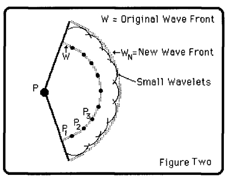
Planar Waves

Planar waves can also be predicted in the following manner. Just as in our golf ball example, small wavelets would rise from points, P1P2P3…... P8 along the original wave front. The only difference is that this time the new wave front forms another plane as demonstrated in Figure Three.

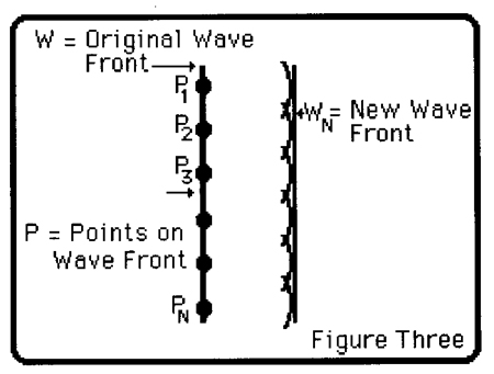
When the number of points, P1P2P3…... P8 is increased to infinity; a very accurate prediction of the resulting new wave front can be determined. The study of calculus permits us to work with many different wave shapes and arrive at complex solutions. Let's apply Huygens' Principle of Superposition to some real-life events.

Listening Through a Keyhole

Did you ever wonder how it was possible to hear a distant conversation through a small keyhole? The answer can be illustrated by examining Figure Four. A sound wave is made to strike a solid door. There is a keyhole slit in the door. W is the original wave front, which in this case is a planar wave. Our new points of origin are concentrated at the outer edge of the keyhole slit. We'll assume that the solid door does not permit the incident wave to reflect and interfere with itself. WN is the new wave front after it "bends" around and through the keyhole slit in the solid door.

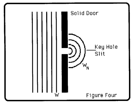
It is interesting to note that as the distance from the keyhole slit increases, the circumference of W8 begins to resemble the original planar wave, W. See Figure Five. The amount of energy that gets through the keyhole slit depends upon the size of the slit as compared to the wavelength of the original sound. This principle should be considered when installing speakers behind perforations.

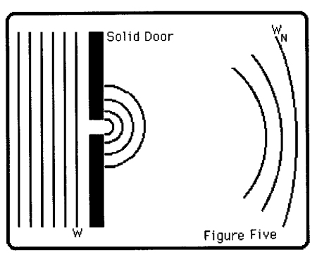
When applying sound deadening material to a surface in a car, it can now be seen why it is important to overlap the individual layers of material. If we leave a small crack in between sections of the deadening material, the sound will get through the crack and try to reform the original vibrations. If overlapping is not practical, the seam should be sealed with something like silicon and then duct tape can be applied over the silicon.

Listening Around Corners

In a similar manner we can apply the Principle of Superposition to the bending of sound waves. This time the points for our new wave front will form a pattern like that of Figure Six. This is how sound waves travel around steering wheels and over consoles. Remember, the new wave front will always try to reform the original wave front. The amount of energy that is "bent" around the corner is again dependent on the wavelength of the sound.

Summing Up

Huygens' Principle of Superposition tells us that as a wave front travels through a medium, a new wave front is formed out in front of the source. This new wave front is the summation of an envelope of wavelets, which spread out from all the many points on the original wave front. With Huygens' principle it is possible to see why many different sounds can be conducted through the same air space at the same time because each wave is unaffected by the others as it travels through the medium. When considering any particular particle in air space, the total energy of multiple sound waves passing that particle at any given point in time, can be given by adding up the energy from the individual sound waves. In an earlier issue of AM we demonstrated that for two identical sine waves, the total energy at any particular point in time must lie somewhere between zero and twice the peak amplitude of either wave.

---

A2538 - Wiring Woofers in Series or Parallel

By Richard Clark

Nothing is more basic than wiring speakers into an audio system. One of the first things any installer or audio enthusiast learns about is the fundamental principle of impedance matching of speakers to amplifiers. Installers learn about the basics of Ohm's law and how series and parallel wiring affects amplifier loading and ultimately, power delivery. And just about the time they start to learn the basics of series and parallel wiring of speakers, they are introduced to the more advanced issue of complex impedance.

When installers first hear about complex impedance and the fact that speaker impedance is really nothing like a simple resistor, they begin to understand that things are not always as simple as we would like them to be. In addition, more often than not, this new awareness leads to misunderstandings that make some things more difficult than they need to be.

After being asked about the subject of series versus parallel wiring of speakers for what seems like the millionth time, and seeing a lot of misinformation posted on the Internet, I felt it might be a good time to cover the topic of speaker wiring. The real issue seems to be that many installers and audiophiles feel that there is some sort of problem with series wiring of speakers and that the only proper way is to keep speakers in parallel.

Since a picture is worth a thousand words, and a measurement is worth at least that many, I thought I would do a series of tests and share the facts about this subject. For the first series of tests, we took four JL Audio 10 inch woofers and carefully measured them in both series and parallel configurations. These woofers were dual voice coil types so for all the tests they were essentially 3-ohm units because we kept the speaker's own internal coils wired in parallel.

First we measured the series and parallel impedance of all four speakers. Figure 1 shows the impedance curves of both configurations. The top curve (black) shows a nominal impedance just under 15 ohms for the four speakers in series -- 4 speakers X 3 ohms each = about 12 ohms. The bottom curve (red) shows the four speakers in parallel.

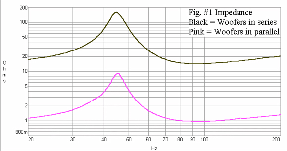
Figure 2 shows the actual acoustic output of the speakers measured outside of a car. Note that the response is smooth for both curves and that they are virtually identical. There is one very small difference, but it is less than a dB for only a few cycles near 45 Hz. Considering the high resolution of the display I would consider this small difference to be near the limits of repeatability of the test setup. In each measurement the actual wattage was exactly the same for each set of four speakers. As can be seen from this test there is virtually no difference in the frequency response performance of a set of speakers wired in series or parallel.

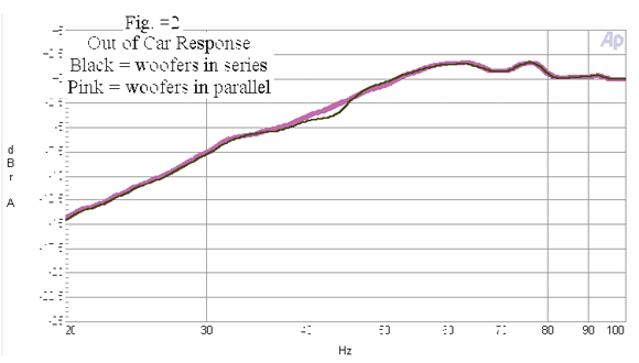
Now it is true that this measurement only covers the steady state performance and the first question raised is usually, “Well, what about damping?” It is true that in the simplest sense of the definition, the damping factor is lessened by a series connection of speakers. Since the definition of damping is simply the ratio of source impedance to load impedance, there would appear to be a big difference. The fact is that damping is not simply a ratio of source to individual speaker impedance, but to the total load -- which is the total impedance of both speakers in series.

So in reality the damping doubles; however, since the impedance doubles, each speaker remains with the same share of effective damping. This is a result of the fact that each speaker generates back EMF, which when shunted by the amp results in a braking force. In a series arrangement, the braking current of each speaker flows through both speakers, so the overall damping is doubled. The result is that the speaker never knows that there is another speaker wired in series with it.

Now there is one exception to this simple explanation. And that is when the series wired speakers are not of the same type or are in different type cabinets. To illustrate this condition, we performed a test of three speakers. One was a large 18-inch woofer in a sealed box, one was a 12-inch woofer in a sealed box, and the third was a 10-inch woofer in a ported box. The brands of the speakers were also different. Figure 3 shows the impedance curves for the three speakers. They are about as different as anyone could find.

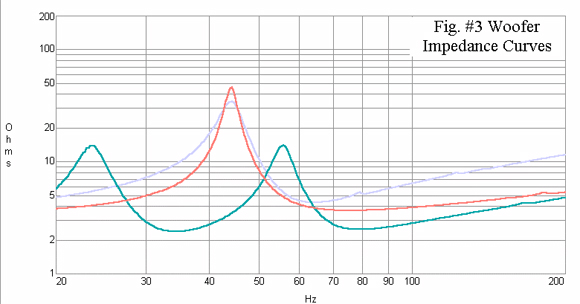
Figure 4 shows the acoustic output of these speakers in different configurations. First is the measurement of only the sealed 18-inch woofer, which we used as a reference. This curve can be seen as the green curve. In this measurement the speaker was wired alone to the amp. Next, we wired the other two speakers in series with the 18-inch woofer. These speakers were placed in another room with long wires so that they would be in the circuit but not contribute any acoustic signal to the 18-inch speaker. The effect of only the electrical signal on the 18-inch can be seen in the black trace. The response remains similar; but there is a loss in level centered at about 55 Hz because of the upper impedance peak of the sealed box being in series with the 18-inch woofer.

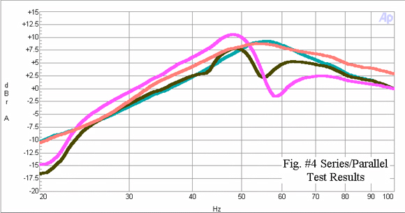
Next we brought all the speakers into the same measurement area and measured the total combined acoustic output of all of them while they were still wired in series. The result can be seen in the pink curve. There is a large loss, about an octave wide, centered at about 58 Hz. In addition, there is a healthy increase of several dB in the octave from 25 to 50 Hz. Of course, these results due to many factors and the actual results would vary greatly depending on the combination of speakers used.

The last measurement is the combined acoustic output with the three different speakers wired in parallel. This can be seen in the red curve. Interesting enough the curve doesn’t vary much from the original curve of the 18-inch woofer by itself. It seems that the 18-inch woofer is dominant over the other smaller speakers, but the combined output does show a slight increase at most frequencies. It is interesting to see that there is not much of a detrimental effect of combining the different speakers in the same system.

So, what’s the conclusion?

1) If the speakers are the same model, then there is no difference in performance if they are wired in series or parallel as long as they are driven with the same total power.

2) If different type speakers are used in the same system, then they may or may not combine in a favorable manner; however, they should be wired in parallel to avoid the interaction of different impedance variations.

---

A2546 - Fusing Stiffening Capacitors

By Richard Clark

There have been quite a few installers and contesters who have called our office requesting a fuse value for their Stiffening Capacitors. Given the large gauge wire used to connect the caps into the power supply of a high-end car audio system, a fuse might seem like a safe idea to the uninformed. However, to anyone with even a casual familiarity with basic engineering theory or elementary physics principles, the concept of fusing an electrolytic capacitor is counterproductive. Let's see why.

Construction Basics

First of all a Stiffening Capacitor is a specially designed two-terminal circuit element. A typical large can cap is constructed of two identical conductive thin metal plates separated by a nonconductive insulator. The two plates are usually assembled parallel to each other and rolled into a round configuration. The last step in the manufacture of a large can cap is the charging process. During this process a surplus of electrons is forced onto one plate, the anode. At the same time a like amount of electrons is removed from the other plate, the cathode.

The net result of this process is the permanent formation of the plates and a "charged" capacitor. A high-quality Stiffening Capacitor will stay in this charged condition for a very long time - months. Only stray leakage from the electrodes and across the dielectric insulating material will cause the slow discharge of the device as the electrons migrate to equilibrium.

The plates are made of a material very similar to aluminum foil. It is not uncommon for the thickness of the plate material to be less than .001 inches. Before the plate material can be used for a Stiffening Capacitor the foil is carefully etched so as to provide more plate surface area and thus more capacitance. The secret of contemporary large-value Stiffening Capacitors like the Monster Cap and IntelliCap lies in the etching process.

How Batteries Work

Batteries are devices that convert chemical energy into electrical energy. Between the plates of a battery, the chemical electrolyte completes the reaction required to MAKE electricity. We repeat, batteries make electricity.

When the chemical reaction has depleted, the battery will no longer make electricity. It is then time to reverse the chemical reaction by putting energy back into the plates of the battery. This process is known as replenishing the electrolyte or simply charging the battery.

If a typical automotive 12-volt storage battery is charged, it has a tremendous capacity for producing electricity. Many hundreds or thousands of amperes can be delivered into very low resistance loads for a relatively long period of time --- up to several minutes. The on-going chemical reaction can produce many free electrons and deliver those electrons to the plates and finally to the terminal of the battery.

This means that automotive 12-volt storage batteries are potentially dangerous in the event of a car wreck in which a positive battery cable happened to get pinched in the chassis or frame of the vehicle. There is no way to shut-off the chemical reaction and it will continue producing electrons until the electrolyte is depleted.

Without an appropriate fuse, the vehicle, as well as its contents, could catch on fire and be destroyed. Fusing one connection at the battery will prevent such mishaps by breaking the circuit. Because batteries are producers of energy they must be fused to protect the vehicle and its contents. The exact ampere value of the fuse should be considerably less than the melt-down current of the car's wiring and slightly more than the worst-case load conditions dictated by the accessories.

How Stiffening Capacitors Work

On the other hand, Stiffening Capacitors only store energy and are not capable of making electricity. The stored energy in a Stiffening Capacitor cannot sustain a large amount of current flow for any long period of time because only a finite number of electrons can be forced onto one plate. Once those electrons are gone, there is no way for a Stiffening Capacitor to produce or generate any more energy because it is only a simple capacitor --- it is not a battery. That is about all there is to say about how a Stiffening Capacitor works.

How Fuses Work

The word fuse comes from the French word "fusez" which means to burn or melt. That is exactly how a fuse works. Many electrons are forced through a relatively small cross-section of conductor and the result is heat. Eventually enough heat is developed across the fuse so that it melts and opens the circuit. Fast acting fuses take fewer electrons per unit time to open than do slow acting (slow-blow) fuses.

How many electrons can a large value Stiffening Capacitor hold? Over what period of time must how many electrons flow to cause a fuse to melt? Well, we conducted a simple experiment to demonstrate the effect of fusing a Stiffening Capacitor.

First we charged a 1 Farad Stiffening Capacitor up to 14-Volts and then placed a fast acting fuse rated at 10-amps directly across the cap's electrodes. The fuse melted with a spark discharge at either electrode. We recharged the Stiffening Capacitor and reached into the 20-amp fuse drawer.

The 20-amp fuse also melted as soon as contact with the Stiffening Capacitor' s electrodes was made. We then recharged the capacitor and tried a 50-amp rated fuse. This 50-amp fuse had a 200,000-ampere peak rating, which means that for a very short period of time, the fuse was capable of sustaining a current flow of incredible proportions. Obviously the Stiffening Capacitor was completely discharged before the fuse element heated up enough to open the circuit. This time the resistance of the fuse was not high enough to melt as the entire flood of electrons (CV2 1 x 142 196 Coulombs) flowed between the plates on their way toward equilibrium. We could have repeated this experiment until an exact fused value was determined, but there is really no reason.

Effect of Fusing a Stiffening Capacitor

The purpose of installing Stiffening Capacitor in a 12-volt automotive sound system is to augment the alternator/battery power supply of the car. The internal impedances associated with an un-stiffened supply commonly cause the power supply to sag and drop out. The ability of a Stiffening Capacitor to deliver instant energy to the power supply of an amplifier prevents dropouts and can improve the quality of the sound system.

Installing a fuse on a lead from a Stiffening Capacitor can limit the ability of the capacitor to deliver its electrons to the sound system. Any fuse that is capable of melting WILL restrict the effectiveness of the Stiffening Capacitor. Any fuse that has a fused rating that is too large to blow with the full output of the cap will probably restrict the effectiveness of the Stiffening Capacitor, AND will also be totally useless as a safety device.

Summing It Up

Fuses are meant as safety devices and are installed as a protection measure. Just like IASCA says, we should always fuse a connection made to a battery. There is no question about this practice. However, fusing a capacitor is another matter. There is no logical argument for such a practice. If an effective fuse is to be installed on a Stiffening Capacitor, then the Stiffening effect of the capacitor will be compromised. How much will it be compromised? Well, you might as well just go ahead and skip the whole idea. How would you like to put out a fire with a three-inch water hose utilizing a one-inch coupling?

Note: Stiffening Capacitor is a trademark of Autosound 2000, Inc and used by permission by Monster Performance Car.

---

A2553 - Power Supply Considerations

By David Navone and Carl Miller

There comes a time when we need a bench supply to test or check out equipment destined to operate from our automotive "12 volt" DC supply. The term "12 volt" is in quotes because we know it is about 12.5 volts with the engine off and about 14.4 volts when the charging system is operating. We can call the “12-volt" a nominal level with the understanding that it can mean anything from 12 volts up to 14.4 volts.

For purposes of discussion, let's say that the required voltage is the usual value of 13.6 volts DC. The quick and easy way to get 13.6 volts is to purchase a good 120 volt AC to 13.6 volt DC power supply. If you are curious about what makes it tick or are considering making your own bench supply, the following items should be considered.

What's Really Important

The following four points will be equally germane regardless of the amperage you may need. Whether you require a simple 3 amp bench supply or a 200 amp display supply, the basics are still the same. Let's choose a modest 12 amp supply capable of delivering about 150 watts.

If we were to put together a bench supply using a transformer rated at 12 amps with 12.5 volts either side of the center tap. The most common complaint would be that the supply wouldn’t hold regulation. See Figure 1.

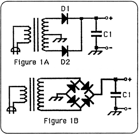
Unfortunately that transformer won't even come close to achieving our goal. Here's why. Notice that diodes D1 and D2 of Figure 1A conduct on alternate cycles. This means that half of the time D1 conducts and the other half of the time diode D2 conducts. A diode drops or looses approximately .7 volts across its terminals; however, with 12 amps of current flowing, the diode drop can exceed 1 volt. That lost volt is associated with some heating of the diode.

I'd like to mention here that Figure 1B illustrates a full wave rectifier. This circuit topology may not require a center-tapped transformer, but the four diodes cause even more of a voltage drop (around 2 volts).

Filtering

After the AC is rectified, it must be filtered. With a current draw of 12 amps, 16,000 mfd at C 1 will yield a ripple of 8.5%. This amounts to a ripple voltage of 1.5 volts. So we lose another 1.5 volts here. (See Figure 2)

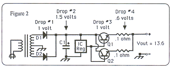
Regulation and Pass Transistors

At this point the IC (Integrated Circuit) regulator usually drives two pass transistors, Q1 and Q2. Although each pass transistor handles 6 amps; there is another 1 volt drop across the base-emitter junction.

Equalizing Resistors

Continuing on with our Figure 2, we notice that there is a .1 Ohm resistor following each pass transistor. These resistors assure that the two pass transistors will equally share the load. Without the equalizer resistors, one transistor would have to work too hard and eventually be destroyed. The bad news here is that with 6 amps flowing through a .1 Ohm resistor, there will be another .6 volt drop.

Adding Up the Drops

Adding up all the voltage drops we notice that they total 4.1 volts. If the output is held at 13.6 volts by the regulator, then the transformer must supply 13.6 volts PLUS another 4.1 volts (rms) with a 12 amp load. This means that we must have a minimum of 17.7 volts. This is why a 12.5-volt transformer will not work for a 12 volt power supply.

---

A2555 - Bass Principles

By Richard Clark

We recently tested a loudspeaker for a manufacturer and ended up with a great opportunity to discuss the basic principles of low frequency response in a car. An understanding of how a low frequency speaker is affected when it is placed in the car can be very helpful in the design of better low frequency systems. A lot has been written about the effect the listening space has on the response of a loudspeaker but little has been published on how this applies to a car. Sometimes the information concerning loudspeakers and a home listening room can be misleading when the information is applied to car audio installations. To clear up some of these problems, let's begin with a subject that we touched upon earlier -- the subject of loudspeaker directivity.

Boundaries and Directivity

A review of the basic directivity behavior of a loudspeaker tells us that if we start with a loudspeaker in a box suspended in air (Figure 1) at wavelengths that are large (relative to the box size) the dispersion pattern of the speaker will be basically omni directional. Since we are only interested in the behavior of woofers, we are going to limit our consideration to low frequencies - after all that is what woofers are for.

If we take that same woofer and enclosure and mount it flush in a large wall (Figure 2), the SPL will increase. The increase in SPL is because the total energy that was once radiating into a complete sphere has now been concentrated into half the space. At higher frequencies (where the wavelengths are short relative to the size of the speaker) this will result in an SPL increase of 3 dB -- a doubling of power. However, at lower frequencies this increase can be as much as 6 dB provided the dimensions of the boundary are large relative to the wavelength.

This large boundary causes a doubling of pressure (not power). This doubling of pressure at the long, in phase wavelengths is what gives us an increase of 6 dB. If another boundary is added (Figure 3), we will see an additional increase of 3 dB. Once again, however, if the boundary is sufficiently large, we can see as much as 6 dB. This would bring the total SPL increase to 12 dB.

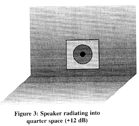
Now adding yet another boundary (we're up to three now, see Figure 4) can add another 3 to 6 dB over our existing value. This is analogous to putting a speaker in the corner of a room. Anyone who has ever experimented with loudspeaker placement in a room quickly learns about the 9 to 18 dB of "free" bass that can result from corner placement.

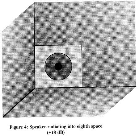
What About Cars?

There are not many technical books published on the subject of bass in cars. We know that most car audio enthusiasts are eager for technical information on this subject. Often they turn to the best sources available for information - home and pro-audio books and articles. Sometimes this type of information can be used in car audio and sometimes it can't.

One of these "can't" times occur with the subject of corner or boundary loading of woofers. Although everything we have discussed so far is totally applicable in a home environment, it is not so in a car. This has led quite a number of people to a mistaken understanding of woofer behavior in a car. To understand this difference, consider the dimensions of a typical home listening room. In order for us to have wave behavior in an environment, there must be a space large enough to support the wave. There must also be a medium for that wave to travel in - in this case air.

Whenever the longest dimension of a space is smaller than a complete wavelength, placing a loudspeaker in that environment and causing it to move at that rate will result in nothing more than an alternating pressure change in that space. The propagation is such that the pressure is equalized in the entire environment by the displacement change in the transducer. Only when the velocity of the speaker movement is increased to a point where the rate of change is faster than the propagation through the environment can we have a wave.

Pressure Zones With No Waves

It is easy to see that the dimensions of the space determine the actual frequency where this occurs. This phenomenon is fully in effect when the longest dimension of the space is equal to 1/2 wavelength. Below this frequency the entire space is a pressure zone. The pressure in this zone is no different than the pressure in any other vessel resulting from a displacement change. This means it will be the same everywhere in the space. The pressure distribution would be no different than that in a balloon -- equal at all points.

What does this mean to our speaker?

1) Unless we can factor the car into our calculations, our computer frequency response simulations are going to be totally wrong.

2) At the wavelengths we are interested in, there are no corners in cars, only a large pressure zone. Compared to the wavelengths produced, below 100 Hz the boundaries are just too confining for it to be any other way.

3) The response of the speaker is not going to be different (at low frequencies) due to different placements.

4) If we are inside this listening space, then we will not be able to localize the source of the pressure because there will be essentially no pressure differential (excluding harmonics) between our two ears.

What Does This Mean?

To see the result of these four facts, let's examine some measurements. A small-ported box (0.28 cubic feet) loudspeaker measured outside of a car can be seen in Figure 5. Notice that the response is similar to what we would expect from a simple ported enclosure. The speaker was low-pass filtered at 120 Hz. The actual computer simulation of this speaker was run on TermPro and the simulation bears close resemblance to the actual measured response as shown in Figure 6. The 120 Hz low-pass filter was not part of this simulation. Notice that the response of both graphs starts to roll off rapidly below 80 Hz.

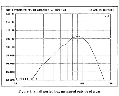
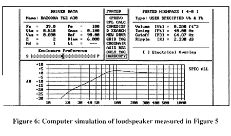
Figure 7 shows the result of placing this speaker inside a sealed car. Notice the tremendous increase in low frequency response below 80 Hz when compared to the computer simulation and the out of car response. This response increase is a result of two factors. Pressure loading from the car concentrates the energy from the speaker into a small-enclosed space. The increase is even higher than what we would expect from corner loading. Second, this higher pressure causes an increase in radiation resistance that actually makes the speaker more efficient. This effect is not that great so we will not concentrate greatly on it.

What happens if we move the speaker to other locations? For the next few measurements we kept the microphone in the same location and moved only the speaker. Notice that only minor variations resulted from moving the speaker. There are some small differences, which are generally at higher frequencies (above 60 Hz) where some modal behavior starts to occur as the wavelengths become shorter.

How audible would these differences be? It can be seen that the peaks and dips that occur between 60 and 120 Hz are all about 1/3 or less of an octave wide. For example, on some measurements there is a dip between 60 and 80 Hz, on others there is a peak between 50 and 60 Hz. One-third octave represents a critical bandwidth. This means that when we listen to the overall response, our brain will integrate the total energy into a curve that contains the points that represent the average energy in each 1/3 octave. So eight data points (20, 25, 31, 40, 50, 63, 80, 100, and 125 Hz) would be used and a line that best fit these points would represent the way we hear the response. This curve is known to mathematicians as a "least squares fit" (LSF). An approximate LSF curve has been drawn as a dotted line through the curves in Figures 14 and 15. Notice that the overall LSF curves do not vary from each other by more than 2 dB. By looking at the LSF represented by all of the previous measurements it can be seen that the low frequency response (below 80 Hz) in a car is not going to vary with box location more than a minor amount. This does not mean that different locations will not produce higher or lower subjective boom between 80 and 200 Hz. This is the range where modal variations begin to occur because the wavelengths start to become small relative to the car size. The varying pressure modes are independent of speaker location and are determined by the size and shape of the interior. If the speaker is located where it radiates into a high-pressure mode, it will be more efficient than if it is placed in a low-pressure mode. Normally, we don't care about woofer response above 80 Hz, and are not concerned with this phenomenon.

---

A2559 - Voltage Dividers

By David Navone

The problem we want to solve is how to get any voltage from a single supply. For instance, let's say that we have a 12 volt DC car battery, but we need to operate a 9 volt DC portable CD player. If we were to use the full 12 volts, we'd probably burn up the little player. Right?

We have discussed in the past what happens when current is passed through two resistors in series. Let's review the schematic symbols for a resistor, R, a potentiometer, and a battery as shown in Figure 1. Notice that the variable resistor, or potentiometer, or pot, has an arrow indicating the wiper or movable contact. This wiper is usually capable of movement throughout the full resistance of the pot: from zero ohms up to the maximum resistance, R. We'll cover potentiometers in greater depth at another time.

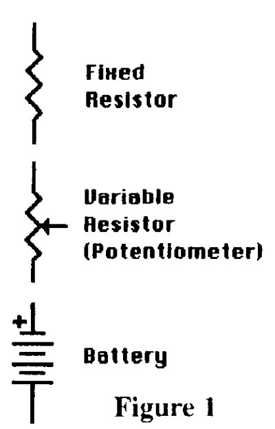
Resistors in Series

As a quick review, refer to Figure 2 which depicts two resistors, R1 and R2 placed in series. Since we're car audio folks here, the potential voltage will be exactly 12.0 volts. Notice that in this case, R I = R2 = 1000 ohms. How much current can flow in such a circuit?

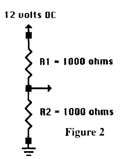
The answer can best be explained in Figure 3 which shows the complete circuit including the 12 volt DC battery, the two 1000 ohm resistors in series, and the current, I. To solve for the current, we use Ohm's Law:

E = IxR, which in this case, E = Electromotive force, in volts, I = Current in amps, and R = Resistance in ohms.

The only tricky part is that in Figure 3, R is really Rt or total resistance. That means that E = IxRt, which can be solved as I = E/Rt, which becomes I = 12 volts/(1000 + 1000) ohms = 12/2000 = .006 amps or 6 milliamps, or 6 mA. So there is 6 milliamps of current flowing through R1 and there is volts 6 milliamps of current flowing through R2.

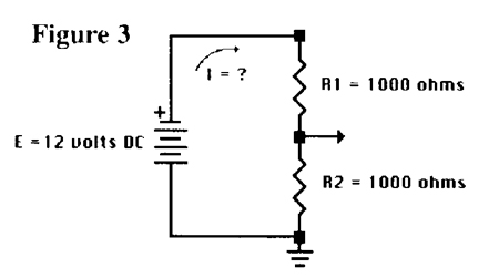
Each resistor must have a 6 volt drop between its terminals. See Figure 4 where E1 = 6 volts and E2 = 6 volts.

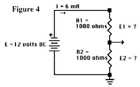
Let's Get Real

But our little CD player needs 9 volts, so how do we calculate that amount? Well, first of all we must determine how much current (at 9 volts) our little portable CD player will draw. This is the most important part of the equation. The best way to determine the current draw of the portable player would be to measure it with a real ammeter. Simply place the meter in series with the power supply and activate the player. Removal of the existing battery pack is recommended. Also be sure to set your meter to some very high scale (i.e. 20 amps) for the initial readings.

Let's say that at 9 volts, the little player draws 900 mA. It may draw a little more current when a CD is starting or when the internal amplifier is required to play low impedance headphones, but we can skip that for now.

So if we know the current through the CD player (.9 amps) and we know the potential across the CD player (El = 9 volts DC), then its resistance, Red, must be:

Red = E/I = 9 volts/ .9amps = 10 ohms. See Figure 5.

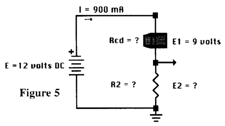
Did we lose anyone yet? We sure hope not because this type of problem occurs quite frequently in car audio. Ok, let's continue.

If the voltage drop across the CD player must be 9 volts, and our supply is 12 volts, then we must find the voltage drop across E2 before we can determine its resistance.

Solving For R2

From Figure 5, it should be apparent that when we subtract 9 volts from our 12 volt supply, we're left with 3 volts. This means that E2 = 3 volts which means that we must drop 3 volts across R2 in order for this circuit to work. See Figure 6.

The drawing in Figure 6 leaves us with only one unknown, the resistance of the dropping resistor, R2. But we know the current flowing in the circuit must be 900 mA, and that we must drop 3 volts across R2, so we can easily solve for R2.

R2 = E/I = 3 volts/.9 amps = 3.33 ohms

So the answer to our question is that we should place a series resistance of 3.33 ohms in our circuit so that we could drop 3 volts from our supply and leave our CD player 9 volts to operate correctly. See Figure 7 for the final solution.

How About the Power?

Before leaving this subject, let's consider the power rating on R2. From Ohm's Law, we know that P = ExI so that means that:

P = (3 volts) x (.9 amps) = 2.7 watts

This is the amount of power that must be dissipated in R2 so that it can drop that all important 3 volts. However, no decent engineer would ever use a 3 watt resistor in such an application. A resistor rated at 3 watts would surely produce quite a bit of heat. Our lowest recommendation would be a 5 watt rated resistor and our best suggestion would be to use 10 watts or higher.

A Basic Question

How do you determine the resistance and minimum power rating required to operate a 12 volt high power car stereo from a 24 volt truck battery? Our bench tests showed that the deck drew 2 amps of current when operated on our 12 volt bench supply.

---

A2594 - RC Time Constant

By David Navone

Not a day goes by without someone calling into our office complaining of some kind of system turn-off noise. Three years ago we wrote an article that basically outlined a simple testing procedure to check for operating noises in amplifiers and other components BEFORE installing them into competition or "high-end" systems. The idea was to give the popping components to someone else. We realize that, however, in the real world of everyday, successful car audio there are two axioms that must be followed:

1) The customer is always right, and

2) The customer is always right.

This means that if there exists any unwanted noises in a system, and changing out or altering components is not a profitable solution, then it is time to step back and objectively evaluate the problem. The point is to get the customer down the road with a minimum expenditure of time and money. Here's one approach to solving the problem of component turn-off pops.

The Concept

Let's say that after using the Autosound 2000 Troubleshooting Flowchart, you've debugged the sound system down to an electronic crossover that exhibits a terrible pop whenever it is turned off. It doesn't matter if the crossover's inputs are muted or there is a signal presents at turn off -- the crossover just pops. Such pops are not uncommon to pro-audio and "high-end" home audio components, but for car audio, the pops can kill a sale and/or lose a contest.

The obvious answer would be to never turn the electronic crossover off. Then we'd never have a turn-off pop. Since that idea has a fatal flaw, we could do the next best thing -- just leave the crossover on for a little while longer. But if we could somehow just leave the crossover on until the amplifiers) were off then we'd never hear the pop. Right?

So that's the idea. We figure out a way to leave the electronic crossover on for a couple of seconds after the amps have shut down. Most car audio components have a "turn-on" lead that activates the component when the 12-volt logic is "high" and deactivates the component when the logic is "low." In installer lingo, put 12 volts on the turn-on lead of a component and it will go on and when the 12 volts is removed, the component will shut down. That means that all we have to do is keep the 12 volts on the turn-on lead of the electronic crossover for a couple of seconds and our problem will be solved.

Time Constant

In basic electricity 101, we learned that a capacitor is a device capable of storing energy. If we had a perfect electrolytic-type capacitor and we charged it up to a potential of 12 volts, those 12 volts would stay there for all eternity. (We charge a capacitor by simply connecting its terminals to a source of EMF (electro-motive force) such as a 12-volt car battery.) After the capacitor's plates are charged and the source of EMF is removed, the capacitor will remain charged.

But in the real world, absorption within the dielectric and the resistance of the air between the capacitor's electrodes will permit some electrons to migrate to the opposite plate and thereby slowly reduce the original potential. The higher the resistance, the longer the capacitor will remain charged.

Also, within every capacitor there is a resistance, R, which is always in series with both the charge and discharge of the capacitor. This is the equivalent series resistance of the capacitor. Refer to Figure 1.

The time constant, T, for a charging capacitor is the time, in seconds, that it takes to place 63% of the charging potential across the capacitor's plates. (Since we usually try to keep advanced mathematics to a minimum, just trust me with the 63% figure.) We must measure the capacitance in farads and the resistance in ohms in order for the time to come out in seconds. The equation for the time constant becomes:

T = RC

Where R = Resistance in Ohms, C = Capacitance in Farads and T = Time Constant in Seconds.

To see how the time constant equation works, let's take the example of a 1000 uF capacitor that is charged through a 680 ohm resistor as shown in the left side of Figure 1. One uF is equal to .000001 farads so 1000 uF is equal to .001 farads. Now that means that T = RC = 680 x .001 = .68 seconds. This means that if we apply 10 volts to a capacitor through a 680-ohm resistor, the plates of the capacitor will reach a potential of 6.3 volts after .68 seconds. Of course, a few seconds later the capacitor will reach the charging potential of the full 10 volts and the time constant equation won't be of any use to us. But hold on...

Using the RC Time Constant

We aren't really interested in the charging time for the capacitor in order to solve our component turn-off problem. We're interested in the discharge time. For instance, if we reapply our equation for 12 volts, we arrive at a discharge voltage of 4.6 volts (after losing 63% of its voltage) in .68 seconds. Don't forget that in order to achieve this discharge rate, we need to use the 680-ohm resistor to "bleed" our capacitor. In this instance, to "bleed" means to drain the voltage through a resistor and dissipate the energy as heat.

So the next big question is how to measure the internal "bleeder" resistance of a component's turn-on circuit. One method is to simply measure the current flowing in the turn-on lead of a particular component. I chose a Soundstream Reference 500 amplifier and measured around 10 mini-amps or .010 amps of current flowing in the turn-on circuit lead. Next, I measured the actual voltage required to activate the turn-on circuitry for that same amplifier. This turn-on cut-off voltage was around 6.6 volts. (A variable bench power supply is great for performing this task.) On this particular amplifier, dropping the turn-on voltage from 14.0 volts down to 6.7 volts did not appreciably change the turn-on current. (There is probably a zener diode in the circuit.) Solving Ohm's Law for R we arrive at R = E/I = 14.0 volts/. 01 amps = 1400 ohms.

However, since the current in the circuit remained constant down to 6.7 volts, let's again calculate the resistance of the circuit. This time R = E/I = 6.7/. 01 = 670 ohms. So for the Soundstream Reference 500 amplifier, the resistance of the turn-on circuitry effectively varies from between 700 ohms up to 1400 ohms. (We'll soon find out that this difference is no big deal.) Let's use an average value of 1000 ohms for the internal "bleeder" resistance of this amplifier's turn-on circuitry.

Practical Application

If we want to leave the Soundstream amp on for one second longer than the rest of the system, then the Time Constant, T + 1 second. By plugging in a value of R – 1000 ohms, and T = 1 second, our T = RC equation can be solved for the capacitance, C. (See Formula 1)

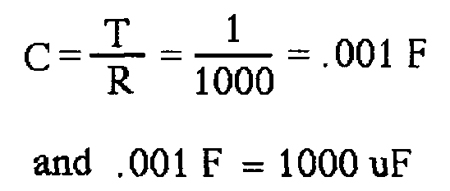
So if we apply a charged 1000 uF capacitor across the turn-on circuitry of the Soundstream Reference 500 amplifier, 14.0 volts of charge potential will get reduced to 37% of its value, or 5.2 volts, in approximately one second. Since 5.2 volts is lower than the 6.7 volts required to turn-on the amp, the 1000 uF capacitor ought to be discharged enough to permit the amp to shut off.

For all of our compulsive subscribers out there, be advised that changing values of R down to 700 ohms (for 6.7 volts) yields a capacitance of 1/700 F or 1500 uF. Changing to a bleeder resistance value of 1400 ohms (for 14.0 volts), yields 1/ 1400 farads or around 700 uF. These values are not a problem for two main reasons:

1) Electrolytic capacitor rated values are usually less than + or - 20 % accurate, and

2) Who cares if the amplifier is left on for one second, two seconds, or even five seconds?

For this situation, I would grab a couple of paralleled 1000 uF, 16 vdc electrolytic capacitors or possibly one 2200 uF or even one 3300 uF capacitor and wire any of them to the turn-on circuit as shown in Figure 2. Note that the area to the right of the dotted line is inside the amplifier.

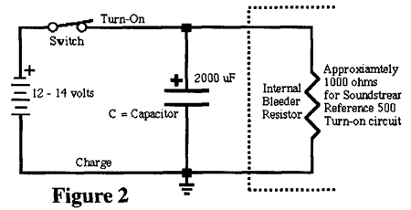
One More Detail

The problem with Figure 2 is that most stereo installers connect all the turn-on leads of all their components together. Our 2000 uF delay capacitance would, of course, now try to keep the entire stereo system on longer. However, because the turn-on circuits would be in parallel, the "bleeder" resistors inside the components would be in parallel and the time constant would have to change. So guess what is now needed? See Figure 3.

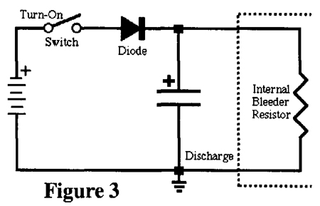
Notice that we have installed a simple diode in series with the turn-on lead of the component that we wish to stay on longer. The band on the diode must connect to the plus (+) capacitor lead. In that way the capacitor will "bleed" down only due to the internal bleeder resistance of that one component.

Summing Up

In summation, the calculations are not critical at all. For instance, if you could only find a 4700 uF capacitor, the Soundstream Reference 500 would stay on for a couple of seconds longer. It is no big deal. Run to Radio Shack and use whatever you can get your hands on. In a tight spot, you can take an inline noise filter apart and use the capacitor. You can take electrolytic capacitors out of broken amplifiers. There is no need to be particular. The diode only has to handle a few volts and practically no current -- any ordinary diode will work.

Using this method it is possible to stagger the turn-on and turn-off of all your components so that they activate one at a time and shut off one at a time. Just measure the turn-on current, determine the cut-off voltage of the turn-on circuit and apply the time constant equation. Give it a try.

---

A2610 - Measuring Magnetic Fields

By David Navone

The reason that cars are noisy is that magnetic fields are created in any region of space where a magnetic force is exerted. For instance, in the region of the alternator, large magnetic forces create the potential needed to charge our starting batteries and operate our 12-volt accessories - including the car stereo system. The last three hundred years of physics have taught us that the strength of the magnetic field is at a maximum when the force on a moving charge is perpendicular (at right angles) to the magnetic field. There is no force when the moving charge is parallel to the field. This means that the magnitude of the force varies between a minimum and maximum, as the moving charge is orientated with respect to the field.

In car audio, the moving charge can be the electrons moving in a signal cable or in a component. Magnetic fields are everywhere, but the car's chassis can be considered as a large plate with its magnetic field stronger nearest the chassis and weaker as the distance between the chassis and the moving charge increases. So the magnitude of the forces exerted upon the moving charge is dependent on the charge's orientation and distance with respect to the field. In practice, we know that if the route of the signal cables is changed, or if the distance between the signal cables and the car's chassis in changed, the level of noise induced into the audio system will be changed. By the way, the "(magnetic) force on the moving charge" translates into alternator whine for car audio systems.

Other low frequency magnetic noises are seat motor pops, windshield wiper motor noise, horn pops, air conditioning motor noise, and side view mirror motor noise. Since the alternator is responsible for producing the greatest changing magnetic field, the alternator creates the largest amount of noise for car audio systems.

In many competition car audio systems, the noise floor of the components must be reduced by as much as 30 dB over regular components. These situations are highly susceptible to induced noise. Also, competition and demo vehicles can include additional electrical accessories (more loads) and higher capacity alternators (more changing magnetic fields). Consider the following questions:

1) Are BMWs with the battery in the back always noisier than regular cars?

2) Is my high output alternator noisier than the stock alternator?

3) How much additional noise is my second battery causing?

4) Will routing the signal cables in the headliner reduce the noise?

5) How much alternator noise is normal?

6) Is there any validity to routing the signal cables away from power cables?

7) How much will the noise drop if a filter cap is placed on the alternator?

8) Will laying the signal cables between the carpet and the pad make a difference?

Calibrated Magnetic Probe

In the lab we use a calibrated magnetic probe to measure the magnitude of a low frequency magnetic field. The probe connects to the input of an oscilloscope or DVM and measures the intensity of the field in mini-volts. The millivolts are then converted to Gauss by the following formula:

Gauss (peak)=84.8•V rmslK•FHz

Vrms is the induced rms voltage measured in millivolts (mV), K is the calibration constant for the individual probe (i.e. I 5.0), F is the frequency of the noise in Hz, and the Peak magnetic field intensity is calculated in Gauss.

Notes: We can assume a frequency, F, of 1 kHz for alternators. This equation is valid for frequencies below 2.5 kHz. Most DVMs will read the magnetic probe's voltage in millivolts rms. Also 1 Gauss = 0.1 milliTesla and 1 milliTesla =10 Gauss. If the probes constant K=15.0, the Frequency= 1 kHz, and the DVM reads 10 mV, the peak magnetic field intensity = [84.8 x 10] / [15.0 x 10001] = 848/15000 = .0565 Gauss.

If you don't like the math, the millivolt output of the probe can be used to map and measure the low frequency magnetic fields of a vehicle. As the millivolts increase so does the magnetic field intensity - they are directly related. The magnetic probe can also be used to find the source of the field. Recall that the field is strongest when perpendicular to the moving charges. The line surrounding the probe indicates the direction of the moving charges. This causes the DVM to read highest when the probe is aimed directly at the source.

The DVM will always read highest when the probe's arrows are orientated towards the source of the field. For instance, when probing the alternator itself, the direction of the magnetic field can be determined by aiming the probe at various places on the case of the alternator. The arrows on the probe point towards the source.

To use the magnetic probe, plug the dual banana plugs into the meter's + and - inputs. Adjust the AC voltage to the scale that reads mV. The case of the alternator is one of the noisiest devices in the car. Observe the DVM as the probe is moved towards the case of the alternator. Most alternators under load will peak at around.5 Gauss. However, it is not unusual to measure high output alternators with magnetic field strengths on the order of 1 Gauss. Thanks to the calibrated probe, you can find out exactly how much noise a high output alternator produces.

To discover if an ECM (engine control module) or vehicle computer could be the source of low frequency magnetic interference, move the probe to the wiring harnesses and case of the control modules. Most such devices radiate noise that is too high in frequency to be read by the probe. It's the low frequency noise that is a problem for car audio because it gets into the signal cables and components and is very difficult to eliminate.

Following are some typical magnetic field values for a car:

Alternator (side) = 30 mV = 0.170 Gauss

Alternator (center) = 45 mV = 0.250 Gauss

Alternator (center) with headlights on = 55 mV = 0.310 Gauss

Negative Battery Post with headlights on = 22 mV = 0.120 Gauss

Positive Power cable leading to Power Amplifiers = 4 mV = 0.023 Gauss

Point on car's chassis with headlights on = 2 mV = 0.011 Gauss

ECM with accessories activated = 2 mV = 0.011 Gauss

Amplifier power supply = 6 mV = 0.034 Gauss

Positive Electrode of Stiffening Capacitor Bank = 10 mV = 0.057 Gauss

What do these numbers mean? Since car audio components are susceptible to magnetic fields, it is a good idea to keep the components, and their cables, away from objects that cause high Gauss measurements. The calibrated probe permits the radiating objects to be quickly identified. Then the magnetic fields can be measured and mapped and finally compared with normal situations.

---

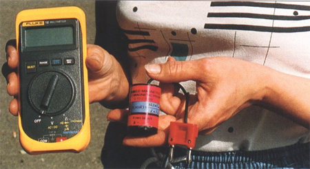
A2625 - Choosing the Right Fuse

By David Navone and Richard Clark

Selecting and installing the correct main power fuse has been a topic of paramount importance for at least the last 15 years. Guided by the rules of competitive autosound, a fuse rating is determined and the master fuse is typically installed within the prescribed distance from the positive battery post. Contests are won and lost over minor variations in this narrow facet of car audio. Each week we receive hundreds of questions about the type, rating, quality, and installation of main power fuses, but seldom do we get asked about the purpose.

Some installers feel that proper fusing at the positive battery post will protect their amplifiers. Others assume that the fuse must be present to save the alternator and battery. However, the majority of installers know that the real purpose of this fuse is to prevent massive current from flowing in the main power cable in the event of a catastrophic event (i.e. a wreck). If the main power cable becomes pinched in the car's chassis, the main power fuse will open and prevent the driver and passengers from burning to death in a fire started by car stereo equipment. For this reason, the car stereo industry has strongly, and appropriately, advised including short circuit protection on the main power lead in the near vicinity of the positive battery post.

Kamikaze Komponent

Fuses are one of our oldest electric components and date back to the times of Faraday, Ampere, Volta, and anyone else involved with the practice of connecting wires to a battery. A main power fuse is a suicide device that self-destructs in order to protect a circuit. The energy in a car's battery is tremendous and is measured in hundreds of amps per hour, which equates to thousands of amps per minute or tens of thousands of amps per second. Since car audio power amplifiers must operate on a nominal 12 volts, the size of the power cables connecting the car's battery to the amplifiers) in a modest system can be #4 AWG or larger. So the question becomes, "What size fuse element will melt open before the #4 AWG wire will turn white hot?"

Recalling that a chain is only as strong as the weakest link, a successful fuse can rightfully be described as the weak link in the power delivery system. We've seen a relatively small 50-amp main power fuse installed on giant competition systems using huge #000 AWG power cable from the positive battery post back to the amp rack. There is always the concern that the main power fuse could be restricting the car audio system. After all, the pencil lead sized fuse element is minuscule in comparison to the power cabling. Perhaps the gold plating on the fuse holder can somehow make up for this problem? To the engineering world, gold plating around a fuse makes about as much sense as gold plating a toilet seat for an outhouse.

High-Tech Fuses?

A fuse is not a high-tech component. We're not saying that catastrophic short circuit protection requires a high-tech device, we're just pointing out that showcasing fuse holders and fuses does little to impress the world outside of car audio. When is the last time a house or building in your neighborhood was wired with a fuse panel? They quit using fuses in homes and buildings sometime in the middle of the last century.

The reason that vehicles are factory wired with fuses is one of economics. Fuses are cheap. What about boats and airplanes? The last time a pilot had to look for a replacement fuse on an airplane was in the 1950s. Even our very first manned space flights in 1961 were devoid of fuses.

Power Wiring in the 2000s

The obvious high tech-replacement for the antiqued fuse is the circuit breaker. Fifty years ago, circuit breakers worked by heating a bi-metallic element that eventually "tripped" a mouse-trap-like switch. The heating element had to cool down before the breaker could be reset. Today, circuit breakers are extremely sophisticated and include a switch so that the main power can be easily controlled while working on a system. Also with circuit breakers, the exposed wiring is minimized.

Types of Circuit Breakers

There are many manufactures of low-voltage circuit breakers that are suitable for car audio applications. One type of breaker is the temperature-independent Hydraulic Magnetic Circuit Breaker that can always carry 100 percent of its rated current but will trip at 125 percent. It works by routing the current over a hermetically sealed solenoid containing an iron core, a spring, and dampening fluid. This breaker can be immediately reset and comes in virtually any size.

Magnetic circuit breakers use a trip mechanism that is triggered by an electromagnet and an armature. As the current exceeds the limit, the magnetic field strength of the electromagnet changes and pulls the armature to trip the breaker. There are combinations of magnetic and thermal breakers that offer the best of both worlds. Monster Performance Car sells these high quality magnetic breakers.

Check it Out

Recently there was some terrible misinformation on the Internet about circuit breaker failures and the superiority of fuses. The article dealt with failure modes resulting in short circuits. After reading the article, we were supposed to drive down to Home Depot and load up on fuses to replace our household breakers. Yeah right! We're not here to sell circuit breakers but if anyone believes that a fuse has any advantage except price, just try selling a fuse to NASA or the military.

If you want to score extra points in competition this year, we highly suggest looking into the latest generation of circuit breakers. (Of course it will take a technical-minded installation judge to recognize the advantages of a circuit breaker.) When more and more competitors choose circuit breakers, the distributors will add housings, monitoring accessories, and remote options. It won't take long for mainstream car audio to begin showcasing circuit breakers in demo cars and magazine layouts. And when we see the first gold-plated circuit breaker accessories, we'll know that car audio has finally arrived in the 2000s.

---

This site contains mature content
Created by REN in Microsoft Visual Studio 2022
Copyright ©2002-2024 Brandywine Engineering    All rights reserved
All other trademarks, logos and graphics are the property of their respective owners
Questions? Comments? Gather your thoughts and compose a message to the assholes in charge